Classical labyrinth generation algorithms. Part 2: Immersion in Accident
Foreword
→ First part
So. Having estimated the response of the Habr audience and sorting out the cases, I set about writing the second article from the cycle. The reaction of the public turned out to be much more positive than my assumptions, which means that we continue the conversation on one of the most interesting procedural generation topics - the creation of labyrinths.
')
In this part we will talk about what a random and pseudo-random generation is, what algorithms can give us equally likely labyrinths in no way similar to each other and what are their disadvantages. The heroes of our today's adventure will be the Wilson algorithm and the Aldous-Broder algorithm for creating a random spanning tree (Uniform Spanning Tree). CAUTION TRAFFIC .
Let us recall what the ideal mazes in question are. If from each vertex of the graph to any other there is exactly one path and it is impossible to pass all the vertices without passing along the same edge twice, then we call such a graph a core tree . If in the maze in question from each cell to any other there is exactly one passage and it is impossible to visit all the cells without going through the same corridor twice, then we say that such a maze is perfect . The meaning does not change for one simple reason - labyrinths are graphs, as I wrote in the last article. If you have not read it yet, I strongly advise you to scroll a little higher, follow the link and get acquainted with it before moving on.
And although the algorithms presented in this part are very slow and “stupid”, they need to be dealt with, since they are the foundation for our entire topic and for all my articles. The main reason why I did not immediately start with them is that Wilson is not very easy to implement and understand for beginners, which does not prevent him from being extremely curious.
Pro lua
In Wilson’s algorithm, and possibly in some others, which I’m going to write about, the next (table [, index]) function is used to select a random cell that has not yet been visited. Her description from the official Lua documentation:
Therefore, instead of selecting a cell with math.random and checking whether it is processed or using a stack of stack cells along with a hash table to track its location, you can use only one hash table, the keys of which will be hashed coordinates and take elements from it using next.
Allows the application to retrieve all fields in the table. The first parameter is the table, the second is the index in this table. next returns the next index in the table and the corresponding value. If the second parameter is nil, next returns the starting index and its associated value. When calling the last index, or with nil in an empty table, next returns nil. If the second parameter is missing, it is interpreted as nil. In particular, you can use next (t) to check for an empty table or not.
Therefore, instead of selecting a cell with math.random and checking whether it is processed or using a stack of stack cells along with a hash table to track its location, you can use only one hash table, the keys of which will be hashed coordinates and take elements from it using next.
key = next(cellsHash, nil) local start_x, start_y = aux.deHashKey(key) cellsHash[key] = nil — , nil / Offset and Accident
What do we mean by random generation? Can we say that if in the second maze, unlike the first, there are no two walls in the south, then they are completely random? Or if the first labyrinth has two horizontal corridors more? Yes and no.
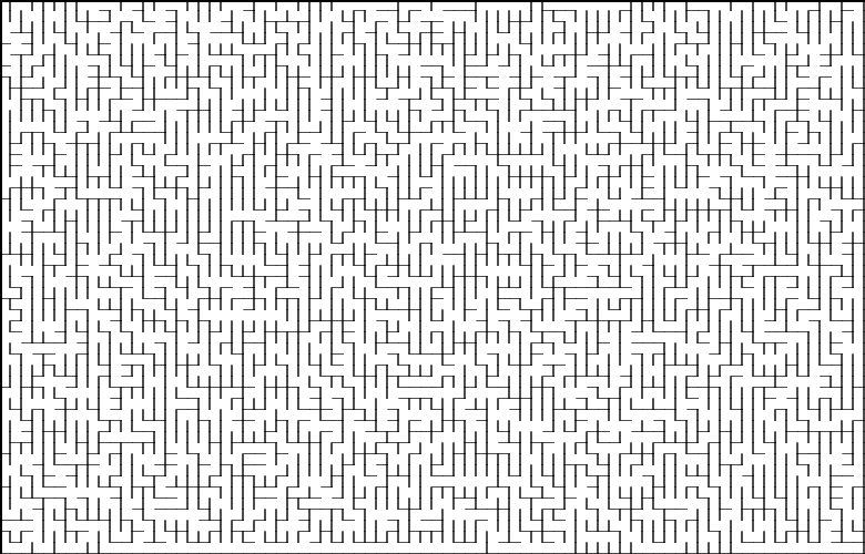
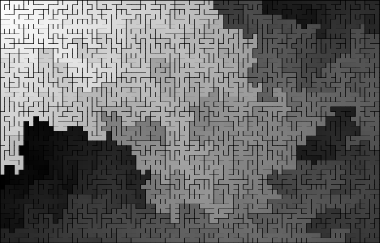
Speaking of randomness in the labyrinths, we must clearly understand what we mean. Let's look at the result of the binary tree algorithm:

As you can see, although the labyrinths themselves are completely different, their displacement is slightly different.
Did we get a random result? Yes. Can we take it as such? Well, in my opinion, no.
The problem is bias (bias), which largely determines the "accident". Algorithms that, by definition, should create random mazes, eventually create similar ones. If “similarity” is pronounced, as in a binary tree, we say that such a maze is easily solved. If, when comparing several labyrinths, it is difficult to unequivocally tell us what the algorithm is about, we say that such a maze is more difficult to solve. To find the displacement, we need to compare several generation results and build a statistical model, according to which we could write a smarter search for the path, or “more intelligent” to solve mazes of this type. For example, we can say that a binary tree algorithm has n times more horizontal passes than vertical ones. This means that it will be possible to take into account the data and speed up the process of finding the exit.
But what if we want the offset to not exist at all? So that, for example, 9 unrelated points of the graph, each time we get a completely different spanning tree? Then we need each of the directions for the algorithm to be equivalent. This means that we allow passing along the vertices already passed, therefore, in each iteration of the cycle we will randomly choose one of four directions, regardless of whether we were there or not. The only condition - do not go beyond the field.
Speaking of the term Uniform Spanning Tree. We already know what a spanning tree is. By connecting all the vertices of the graph with edges so that it is impossible to get from any vertex to another without passing the same edge twice, we get a spanning tree. But if there are more than two vertices in the graph, then there can be more tree variations, right? So, Uniform Spanning Tree is one equally selected variation of a spanning tree in a certain graph.
So. We want completely random labyrinths completely different from each other, and are even ready to sacrifice speed. Then let's get acquainted with the Aldous-Broder and Wilson algorithms.
Aldous-Brodera Algorithm
Description
Remember I said that the binary tree algorithm is the easiest to understand? So, I'm cunning. It is really simpler to implement, since there we always deal with only one direction and one considered row, but the Aldous-Broder algorithm went far ahead in primitiveness and “stupidity”. Its whole meaning is to wander aimlessly around the field, hoping to stumble upon the top of the spanning tree being created and attach another, and then again randomly select a point in the maze and walk until we get into one of the connected ones.
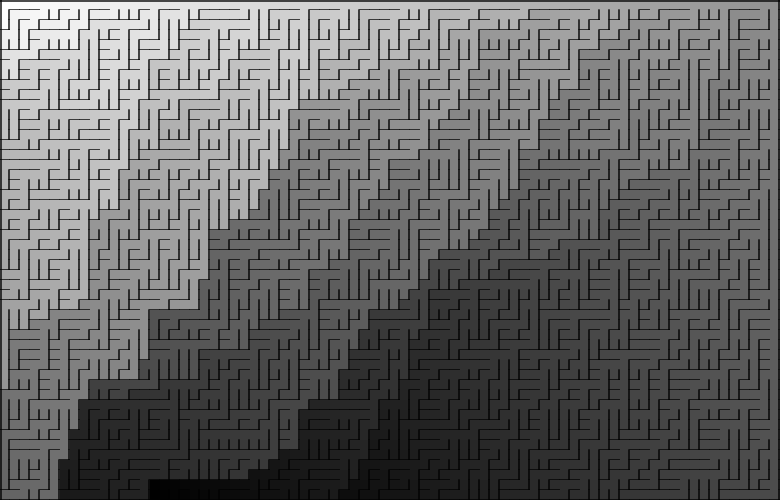
Aldous-Broder is free from any bias. Perfectly. All the labyrinths obtained with its help are completely random and not similar to each other. The algorithm has no preferences for focus, entanglement, or any other characteristics. The resulting labyrinths are random and equiprobable.
The problem may be the imperfection of random number generators, which themselves can cause any values and produce them more often. But if you use, for example, a randomness generator based on natural noise (wind, decay of uranium), then, perhaps, you can finally fully enjoy the work of the algorithm.
Admittedly, the observation of his work truly gives an awareness of all the perishability and meaninglessness of being. To write a gif with his animation, I spent a lot of time, because I didn’t want to keep within 30 seconds in a 5 × 5 field. When it was necessary to connect only one last unchecked cell to the spanning tree, Aldous-Broder would go to another corner and wind circles there. It was necessary to significantly increase the speed of animation and reduce the field, so that, finally, he managed to bypass all the cells of the maze.
It was created by two independent researchers who studied equally probable variants of spanning trees: David Aldous, a professor at the University of California, Berkeley, and Andrei Broder, a scientist who now works at Google. It is difficult to say unequivocally in which area these studies would be useful. However, besides labyrinths, the algorithm often emerges in works on mathematical probability, which, however, is not surprising, given the principle of its operation.
Formal algorithm:
- Select a random vertex (cell). Absolutely random;
- Select a random adjacent vertex (cell) and go into it. If it has not been visited, add it to the tree (connect with the previous one, remove the wall between them);
- Repeat step 2 until all cells are visited.
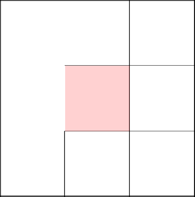
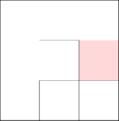
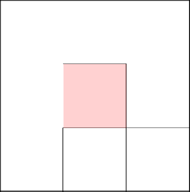
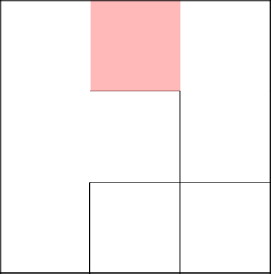
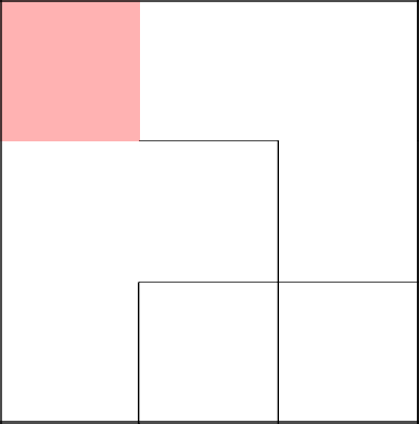
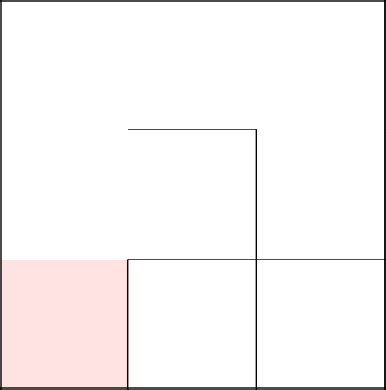
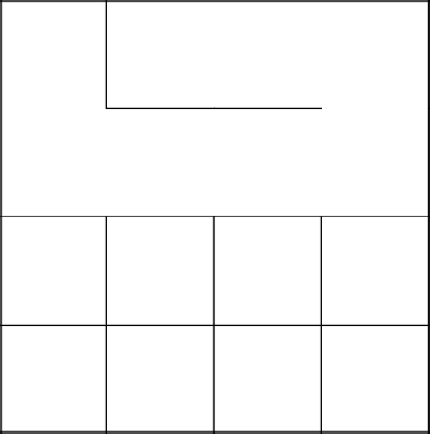
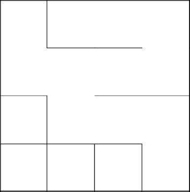
Work example
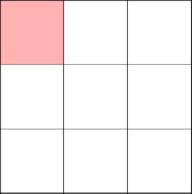
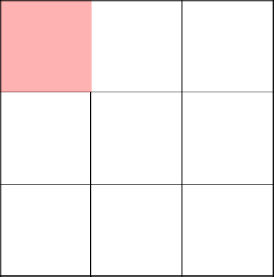
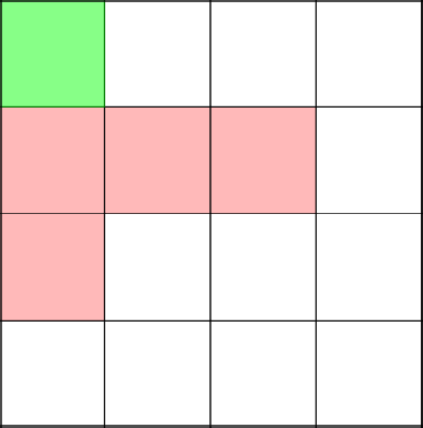
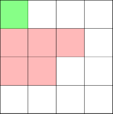
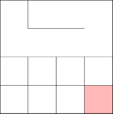
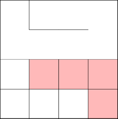
The red color highlights our current position on the field.
Starting from the upper left corner. There is nothing unusual.
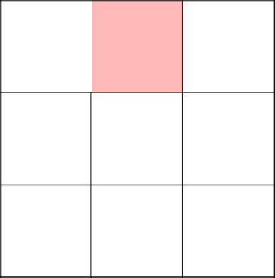
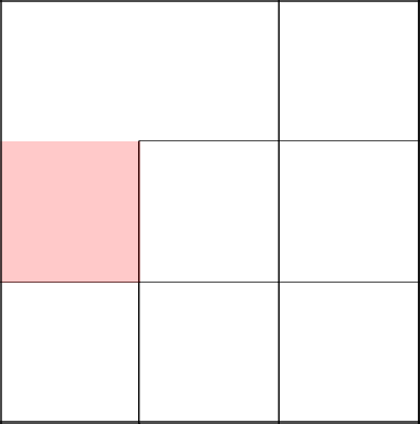
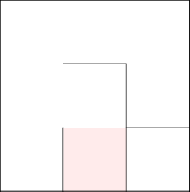
Randomly decide to go to the right and remove the wall between the two cells. Good, we do.
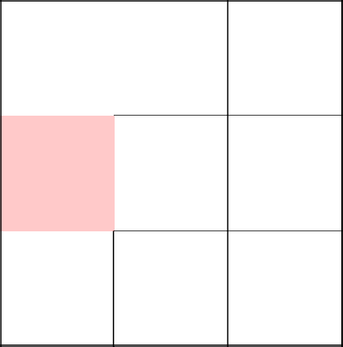
Bad luck. Our RNG tells us to go back, that is, to the left.
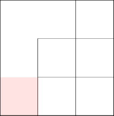
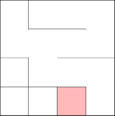
And now down. Along the way, we connect all the unvisited cells and remove walls between them.
Once again lucky. Way down!
Okay, one return can be forgiven.
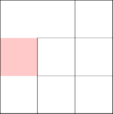
We choose to go to the right and remove the wall.
And here we are twice unlucky and we return to the very beginning.
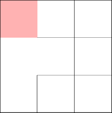
The choice fell twice to the right. Great, at least some variety.
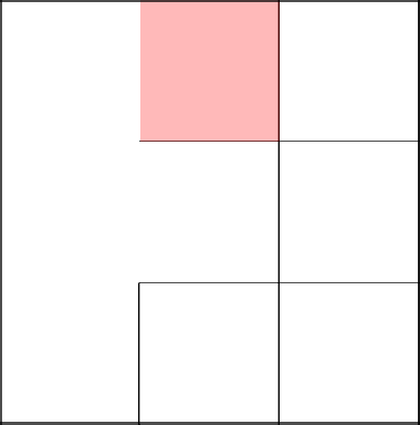

Go down below and remove the wall.
And here, although we are moving to the next cell, we don’t remove the wall, since they are already in the same tree.
It's time to wander aimlessly, walk.

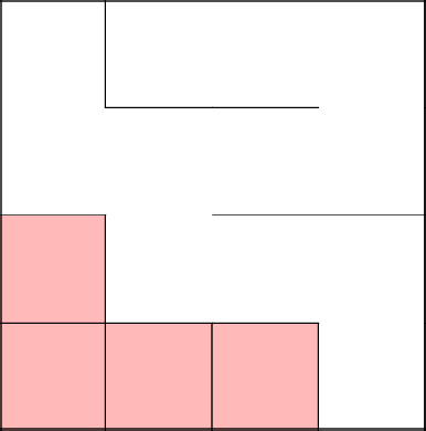
We return to the cage 2-2 and descend below, removing the wall.
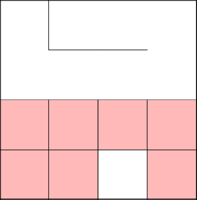
We finish our walk and get the generated maze.
Starting from the upper left corner. There is nothing unusual.
Randomly decide to go to the right and remove the wall between the two cells. Good, we do.
Bad luck. Our RNG tells us to go back, that is, to the left.
And now down. Along the way, we connect all the unvisited cells and remove walls between them.
Once again lucky. Way down!
Okay, one return can be forgiven.
We choose to go to the right and remove the wall.
And here we are twice unlucky and we return to the very beginning.
The choice fell twice to the right. Great, at least some variety.
Go down below and remove the wall.
And here, although we are moving to the next cell, we don’t remove the wall, since they are already in the same tree.
It's time to wander aimlessly, walk.
We return to the cage 2-2 and descend below, removing the wall.
We finish our walk and get the generated maze.
Pros:
- There is no offset;
- Labyrinths are absolutely random, so it is impossible to create a specific algorithm for solving them;
- The complexity of the solution for the person;
- Simple implementation;
Minuses:
- Speed. While the maze is generated, you will have time to grow old and die;
- Does not allow to generate endless labyrinths;
- A strong drop in efficiency at the end of generation;
Implementation
local mod = {} local aux = {} aux.width = false aux.height = false aux.sx = false aux.sy = false aux.grid = false aux.dirs = {"UP", "DOWN", "LEFT", "RIGHT"} function aux.createGrid (rows, columns) local MazeGrid = {} for y = 1, rows do MazeGrid[y] = {} for x = 1, columns do MazeGrid[y][x] = {visited = false, bottom_wall = true, right_wall = true} end end return MazeGrid end function mod.createMaze(x1, y1, x2, y2, grid) aux.width, aux.height, aux.sx, aux.sy = x2, y2, x1, y1 aux.grid = grid or aux.createGrid(y2, x2) aux.aldous_broder() return aux.grid end function aux.aldous_broder() local unvisited_cells = aux.width * aux.height local ix = math.random(aux.sx, aux.width) local iy = math.random(aux.sy, aux.height) aux.grid[iy][ix].visited = true unvisited_cells = unvisited_cells - 1 while unvisited_cells ~= 0 do local dir = aux.dirs[math.random(1, 4)] if dir == "UP" then if iy-1 >= aux.sy then if aux.grid[iy-1][ix].visited == false then aux.grid[iy-1][ix].bottom_wall = false aux.grid[iy-1][ix].visited = true unvisited_cells = unvisited_cells - 1 end iy = iy-1 end elseif dir == "DOWN" then if iy+1 <= aux.height then if aux.grid[iy+1][ix].visited == false then aux.grid[iy][ix].bottom_wall = false aux.grid[iy+1][ix].visited = true unvisited_cells = unvisited_cells - 1 end iy = iy+1 end elseif dir == "RIGHT" then if ix+1 <= aux.width then if aux.grid[iy][ix+1].visited == false then aux.grid[iy][ix].right_wall = false aux.grid[iy][ix+1].visited = true unvisited_cells = unvisited_cells - 1 end ix = ix+1 end elseif dir == "LEFT" then if ix-1 >= aux.sx then if aux.grid[iy][ix-1].visited == false then aux.grid[iy][ix-1].right_wall = false aux.grid[iy][ix-1].visited = true unvisited_cells = unvisited_cells - 1 end ix = ix-1 end end end end return mod Wilson's algorithm

Description
Congratulations, we finally got to something more serious. Wilson's algorithm is much more complicated than all the previous ones, both in implementation and in understanding. The goal of Wilson, like his more stupid partner Aldous-Broder, is the generation of an equally probable random spanning tree. And although the principle of work is somewhat similar, the details are very different.
The algorithm is still based on the equally probable random selection of the side of movement in the maze (graph), with two important differences:
Moving across the field, we “memorize” all the vertices that we visited until the vertex of the spanning tree was found. As soon as we stumble upon an already added vertex, we add the resulting subgraph (branch) to our generated tree. If a loop is created in a subgraph, then delete it. By a cycle, I mean connecting a vertex that is already in a temporary subgraph with it, but at a different point. In other words, there should not be vertices with more than 2 edges. If you don’t understand now, it’s not scary - then you’ll see it through the example of work.
After the subgraph is attached to the spanning tree, the choice of the next random point comes exclusively from the not yet connected vertices. Consequently, unlike Aldous-Brodera, Wilson is deprived of the disadvantage of aimless wandering around the already processed vertices.
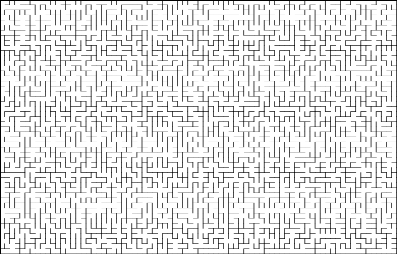
Wilson’s algorithm, like Aldos-Broder, generates completely random mazes without any bias. The algorithm has no preferences for focus, entanglement, or any other characteristics. Unfortunately, to obtain the best results, you should use hardware random number generators that do not have preferences in numbers.
The algorithm itself was published by David Wilson in 1996 in his work on the generation of equally probable random spanning trees. As before, in addition to labyrinths, materials pop up on various websites devoted to mathematical probabilities. Moreover, I happened to stumble upon several interesting publications, concerning the Uniform Spanning Tree and the Wilson algorithm in particular. If in one of them the algorithm itself is described more, in the other as a whole the concept itself and the mathematical basis of the spanning trees are described.
If readers are interested, perhaps I will write part 2a, where I will give the works themselves and their partial translation. The main reason why I avoid the mathematical justification here is my articles are aimed at beginners and people who find programming more interesting than dry math.
Formal algorithm:
- Select a random vertex not belonging to the spanning tree and add it to the tree;
- Select a random vertex that does not belong to the spanning tree and start traversing the graph (labyrinth) until we arrive at the already added vertex of the tree; If a cycle is formed, delete it;
- Add all vertices of the resulting subgraph to the spanning tree;
- Repeat steps 2-3 until all vertices are added to the spanning tree.
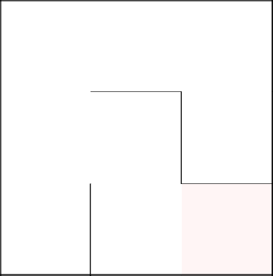
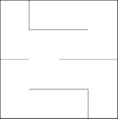
Work example
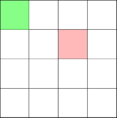
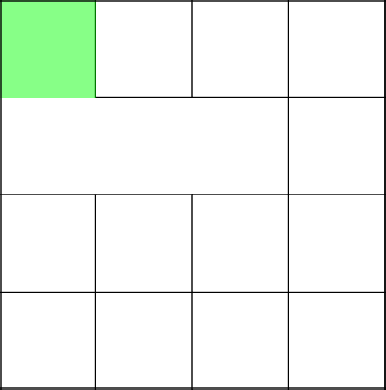
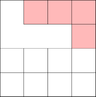
Green highlights the first top of the tree. Red - created branch (subgraph).
Traditionally, you need to get to the upper left corner. We start to build a branch with a 3-2 coordinate.

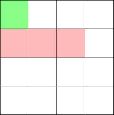
Here is an interesting and important point. The algorithm decides to go up, thereby closing the branch in the coordinate 2-2.
Remove the resulting cycle and start with a 2-2 build again.

habrastorage.org/files/e9c/8e6/46a/e9c8e646af564a42bbb391fbe263044b.png
Well, the algorithm decided to go upstairs and thus joined the main tree. We remove the walls on the way and select the next cell.
Again, we touched a newly created tree, removed the walls and started anew.
Locked, removed the cycle, continued with 2-3 again.

Joined with a tree, cleared the way from the walls. We continued our journey in a new cage.
Again connected with the main tree, removed the walls, finished the labyrinth.
Traditionally, you need to get to the upper left corner. We start to build a branch with a 3-2 coordinate.
Here is an interesting and important point. The algorithm decides to go up, thereby closing the branch in the coordinate 2-2.
Remove the resulting cycle and start with a 2-2 build again.
habrastorage.org/files/e9c/8e6/46a/e9c8e646af564a42bbb391fbe263044b.png
Well, the algorithm decided to go upstairs and thus joined the main tree. We remove the walls on the way and select the next cell.
Again, we touched a newly created tree, removed the walls and started anew.
Locked, removed the cycle, continued with 2-3 again.
Joined with a tree, cleared the way from the walls. We continued our journey in a new cage.
Again connected with the main tree, removed the walls, finished the labyrinth.
Pros:
- There is no offset;
- Labyrinths are absolutely random, so it is impossible to create a specific algorithm for solving them;
- The complexity of the solution for the person;
- No pointless wandering;
- The speed compared with Aldous-Broder many times more;
Minuses:
- Difficult implementation;
- Speed drops at the beginning of generation;
- Greater memory requirements than Aldous-Broder;
Implementation
local mod = {} local aux = {} aux.width = false aux.height = false aux.sx = false aux.sy = false aux.grid = false aux.dirs = {"UP", "DOWN", "LEFT", "RIGHT"} function aux.createGrid (rows, columns) local MazeGrid = {} for y = 1, rows do MazeGrid[y] = {} for x = 1, columns do MazeGrid[y][x] = {visited = false, bottom_wall = true, right_wall = true} end end return MazeGrid end function mod.createMaze(x1, y1, x2, y2, grid) aux.width, aux.height, aux.sx, aux.sy = x2, y2, x1, y1 aux.grid = grid or aux.createGrid(y2, x2) aux.wilson() return aux.grid end function aux.hashKey(x, y) return x * aux.height + (y - 1) end function aux.deHashKey(value) return math.floor(value/aux.height), value%aux.height + 1 end function aux.hashCells(grid) local vtable = {} for yk, yv in pairs(grid) do for xk, xv in pairs(yv) do if xv.visited == false then vtable[aux.hashKey(xk, yk)] = xv end end end return vtable end function aux.wilson() local cellsHash = aux.hashCells(aux.grid) -- , local dirsStack = {} -- local dsHash = {} local dsSize = 0 -- local key, v = next(cellsHash, nil) v.visited = true cellsHash[key] = nil while next(cellsHash) do -- , key = next(cellsHash, nil) -- local start_x, start_y = aux.deHashKey(key) local ix, iy = start_x, start_y while not aux.grid[iy][ix].visited do -- , local dir = aux.dirs[math.random(1, 4)] local isMoved = false key = aux.hashKey(ix, iy) if dir == "UP" and iy-1 >= aux.sy then iy = iy - 1 isMoved = true elseif dir == "DOWN" and iy+1 <= aux.height then iy = iy + 1 isMoved = true elseif dir == "LEFT" and ix-1 >= aux.sx then ix = ix - 1 isMoved = true elseif dir == "RIGHT" and ix+1 <= aux.width then ix = ix + 1 isMoved = true end if isMoved then -- , if dsHash[key] then -- dirsStack[dsHash[key]].dir = dir for i = dsHash[key]+1, dsSize do local x, y = aux.deHashKey(dirsStack[i].hashref) dsHash[dirsStack[i].hashref] = nil dirsStack[i] = nil dsSize = dsSize - 1 end else local x, y = aux.deHashKey(key) -- dsSize = dsSize + 1 dsHash[key] = dsSize dirsStack[dsSize] = {dir = dir, hashref = key} end end end for i = 1, dsSize do -- aux.grid[start_y][start_x].visited = true cellsHash[aux.hashKey(start_x, start_y)] = nil aux.grid[start_y][start_x].point = false local dir = dirsStack[i].dir if dir == "UP" then aux.grid[start_y-1][start_x].bottom_wall = false start_y = start_y - 1 elseif dir == "DOWN" then aux.grid[start_y][start_x].bottom_wall = false start_y = start_y + 1 elseif dir == "LEFT" then aux.grid[start_y][start_x-1].right_wall = false start_x = start_x - 1 elseif dir == "RIGHT" then aux.grid[start_y][start_x].right_wall = false start_x = start_x + 1 end end dsHash, dirsStack, dsSize = {}, {}, 0 -- end end return mod Epilogue:
Summing up all the above, it is worth noting that although we got to more complex algorithms and dealt with some new (for someone) graph concepts, the main difficulties are still ahead. The unclearly convoluted algorithms of Eller, Kraskal and Prima, based solely on working with graphs and trees, provide us with difficult, if interesting, publications. However, before you start writing them, you should look at the search algorithms with the return and something called "Catch & Kill", whose work on the generation of the maze is very different from all the others. I gave a hint on the topic of the next article.
What else. In the comments to the previous part, some people asked or threw off their generation algorithms, which was extremely entertaining and joyful. If you once realized the creation of labyrinths in your own invented way and can now remember it - please share. Perhaps, with your permission, in any of the articles I will write about him. In general, I am glad to any interesting stories and memories on the subject. It doesn’t matter if you remember how you drew mazes in a tetrad at school or on a computer at a university.
Well, and as always. Wishes, criticism, comments are always welcome and if you like the topic and want to see the next part, write about it in the comments.
Sources of algorithms on Lua + render on Love2D (the code is laid out at the request in the comments. Did not react):
Github
Source: https://habr.com/ru/post/321210/
All Articles