Data Oriented Design in practice
Recently, an increasingly interesting discussion of an interesting, but not very popular paradigm - the so-called Data Oriented Design ( DOD ). If you are looking for a job with high performance computing, be prepared for the relevant questions. But I was very surprised to hear that some of my colleagues had not heard of this approach and, after a short discussion, were skeptical about it. In this article I will try to compare the traditional OOP approach with the DOD .
This article was conceived as an attempt to compare different approaches without trying to explain their essence. On Habré there are several articles on the topic, for example this . It is also worth watching the video from the CppCon conference. But in a nutshell, DOD is a way to handle data in a cache-friendly manner. It sounds incomprehensible, the example will explain better.
The second test runs 30% faster (in VS2017 and gcc7.0.1). But why?
The size of the
')
The example above clearly demonstrates the advantages of using SoA (Struct of Arrays) instead of AoS (Array of Structs), but this example is from the
To understand the reality of the approach, I decided to write a more or less complex code using both techniques and compare the results. Let it be a 2d simulation of solids - we will create N convex polygons, set the parameters - mass, velocity, etc. and see how many objects we can simulate staying at around 30 fps.
The source code for the first version of the program can be taken from this commit . Now we will briefly go over the code.
For simplicity, the program is written for Windows and uses DirectX11 for rendering. The purpose of this article is to compare the performance on the processor, so we will not discuss the graphics. The
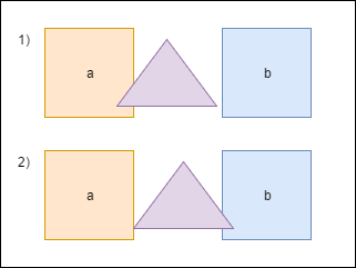
When the triangle intersects with a , we have to move it a little to prevent the shapes from overlapping each other. We also need to recalculate
The heart of our program is the
Each frame we call the
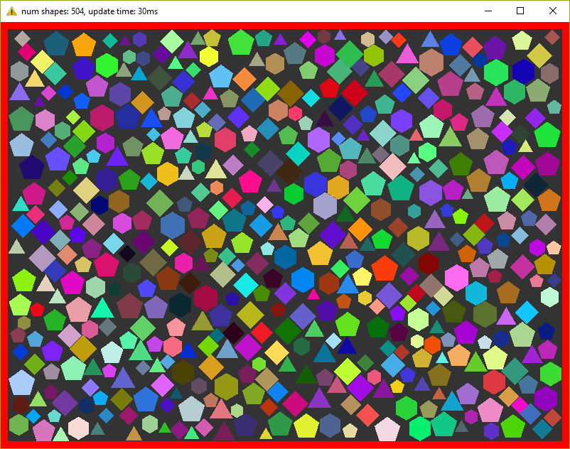
On my old laptop, this program counts 500 figures maximum, before fps starts to fall below 30. Fuuuu, only 500 ???! I agree a little, but do not forget that every frame we repeat the calculations 20 times.
I think that it is necessary to dilute the article with screenshots, so here:
I mentioned that I want to conduct tests on a program as close as possible to reality. What we have written above is not used in reality - to check every figure with each sooo slowly. To speed up the calculations, a special structure is usually used. I propose to use an ordinary 2d grid - I called it a
The commit of the second version of the program can be viewed here . A new
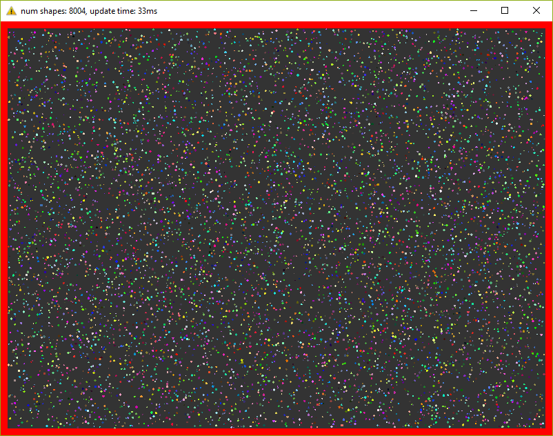
This version already holds 8000 figures at 30 fps (do not forget about 20 iterations in each frame)! I had to reduce the figures 10 times so that they fit in the window.
Today, when even on phones processors with four cores are installed, it is just silly to ignore multi-threading. In this last optimization, we will add a pool of threads and divide the main tasks into equal tasks. So, for example, the
The separation of the main tasks added a bit of headache. For example, if a shape intersects the border of a cell in a grid, then it will be located simultaneously in several cells:
Here the figure a is in one cell, whereas b is immediately in four. Therefore, access to these cells must be synchronized. You also need to synchronize access to some fields of the
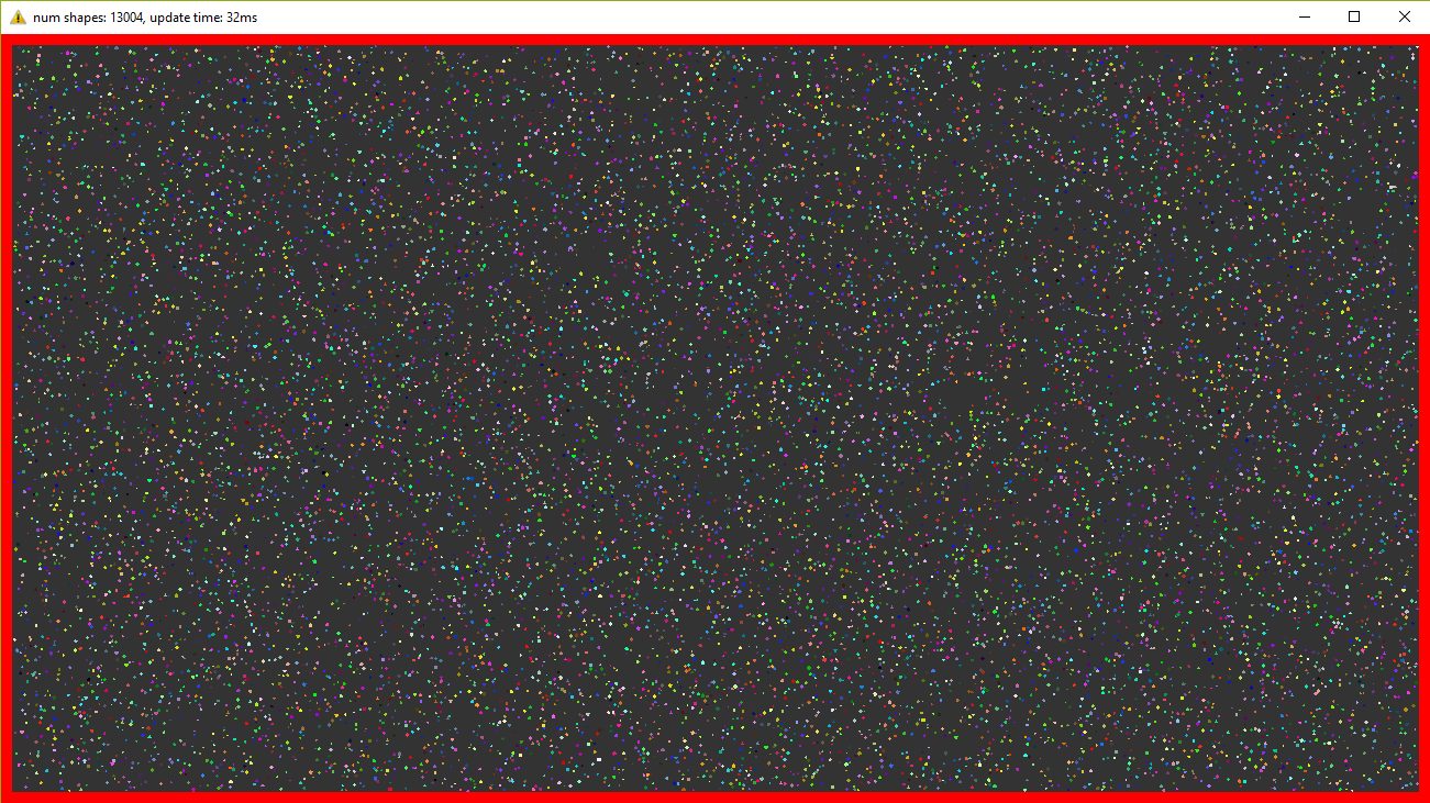
By running this version I can observe 13,000 figures at 30 fps. For so many objects had to increase the window! And again - in each frame we repeat the simulation 20 times.
What we have written above I call the traditional approach - I have been writing such code for many years and I read mostly similar code. But now we kill the
And we pass this structure like this:
Those. instead of specific figures, their indices are transferred and in the method the necessary data is taken from the desired vectors.
This version of the program produces 500 figures at 30 fps, i.e. does not differ from the very first version. This is due to the fact that measurements are carried out on a small amount of data and, moreover, the heaviest method uses almost all fields of the structure.
Further, without pictures, because they are exactly the same as they were before.
Everything is as before, we only change AoS to SoA . The code is here . The result is better than before - 9,500 figures (there were 8,000), i.e. The performance difference is about 15%.
Again, take the old code, change the structure and get 15,000 figures at 30 fps. Those. performance gain of about 15%. The source code for the final version is here .
Initially, the code was written for myself in order to test various approaches, their performance and convenience. As the results showed, a small change in the code can give a rather tangible increase. And it may not give, maybe even the opposite - the performance will be worse. So for example, if we need only one copy, then using the standard approach we will read it from memory only once and we will have access to all fields. Using the structure of vectors, we will have to query each field individually, having a cache-miss for each request. Plus, the readability deteriorates a bit and the code becomes more complicated.
Therefore, it is impossible to answer unequivocally whether it is worth switching to a new paradigm for everyone. When I was working on a game engine on a game engine, a 10% performance boost is an impressive number. When I wrote custom launcher-type utilities, using the DOD approach would only be puzzling to my colleagues. In general, profile, measure and draw conclusions yourself :).
What is DOD?
This article was conceived as an attempt to compare different approaches without trying to explain their essence. On Habré there are several articles on the topic, for example this . It is also worth watching the video from the CppCon conference. But in a nutshell, DOD is a way to handle data in a cache-friendly manner. It sounds incomprehensible, the example will explain better.
Example
#include <chrono> #include <iostream> #include <vector> using namespace std; using namespace std::chrono; struct S { uint64_t u; double d; int i; float f; }; struct Data { vector<uint64_t> vu; vector<double> vd; vector<int> vi; vector<float> vf; }; int test1(S const & s1, S const & s2) { return s1.i + s2.i; } int test2(Data const & data, size_t const ind1, size_t const ind2) { return data.vi[ind1] + data.vi[ind2]; } int main() { size_t const N{ 30000 }; size_t const R{ 10 }; vector<S> v(N); Data data; data.vu.resize(N); data.vd.resize(N); data.vi.resize(N); data.vf.resize(N); int result{ 0 }; cout << "test #1" << endl; for (uint32_t i{ 0 }; i < R; ++i) { auto const start{ high_resolution_clock::now() }; for (size_t a{ 0 }; a < v.size() - 1; ++a) { for (size_t b{ a + 1 }; b < v.size(); ++b) { result += test1(v[a], v[b]); } } cout << duration<float>{ high_resolution_clock::now() - start }.count() << endl; } cout << "test #2" << endl; for (uint32_t i{ 0 }; i < R; ++i) { auto const start{ high_resolution_clock::now() }; for (size_t a{ 0 }; a < v.size() - 1; ++a) { for (size_t b{ a + 1 }; b < v.size(); ++b) { result += test2(data, a, b); } } cout << duration<float>{ high_resolution_clock::now() - start }.count() << endl; } return result; } The second test runs 30% faster (in VS2017 and gcc7.0.1). But why?
The size of the
S structure is 24 bytes. My processor (Intel Core i7) has 32KB cache per core with 64B cache line (cache line). This means that when requesting data from memory, only two S structures will fit completely into one cache line. In the first test, I read only one int field, i.e. with one memory access in one cache line there will be only 2 (sometimes 3) fields we need. In the second test, I read the same int value, but from a vector. std::vector guarantees consistency of data. This means that when accessing the memory in one cache line there will be 16 ( 64B / sizeof(int) = 16 ) values we need. It turns out that in the second test, we turn to memory less often. A memory reference is known to be a weak link in modern processors.')
How are things in practice?
The example above clearly demonstrates the advantages of using SoA (Struct of Arrays) instead of AoS (Array of Structs), but this example is from the
Hello World category, i.e. far from real life. In real code, there are a lot of dependencies and specific data that may not give a performance boost. In addition, if in the tests we address all fields of the structure, there will be no difference in performance.To understand the reality of the approach, I decided to write a more or less complex code using both techniques and compare the results. Let it be a 2d simulation of solids - we will create N convex polygons, set the parameters - mass, velocity, etc. and see how many objects we can simulate staying at around 30 fps.
1. Array of Structures
1.1. The first version of the program
The source code for the first version of the program can be taken from this commit . Now we will briefly go over the code.
For simplicity, the program is written for Windows and uses DirectX11 for rendering. The purpose of this article is to compare the performance on the processor, so we will not discuss the graphics. The
Shape class, which represents the physical body, looks like this:Shape.h
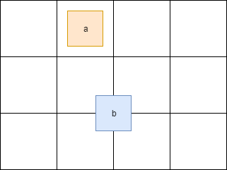
class Shape { public: Shape(uint32_t const numVertices, float radius, math::Vec2 const pos, math::Vec2 const vel, float m, math::Color const col); static Shape createWall(float const w, float const h, math::Vec2 const pos); public: math::Vec2 position{ 0.0f, 0.0f }; math::Vec2 velocity{ 0.0f, 0.0f }; math::Vec2 overlapResolveAccumulator{ 0.0f, 0.0f }; float massInverse; math::Color color; std::vector<math::Vec2> vertices; math::Bounds bounds; }; - The purpose of
positionandvelocity, I think, is obvious.vertices- the vertices of the figures given randomly. boundsis a bounding box that completely contains a shape — it is used to pre-check intersections.massInverseis a unit divided by mass - we will use only this value, therefore we will store it, instead of mass.color- color - used only when rendering, but stored in a copy of the figure, set randomly.overlapResolveAccumulatorsee explanation below.
When the triangle intersects with a , we have to move it a little to prevent the shapes from overlapping each other. We also need to recalculate
bounds . But after moving, the triangle intersects another figure - b , and again we have to move it and recalculate the bounds again. Notice that after the second movement, the triangle will again be above the a figure. To avoid recalculations, we will store the amount by which the triangle should be moved in a special accumulator — overlapResolveAccumulator — and later we will move the shape to this value, but only once.The heart of our program is the
ShapesApp::update() method. Here is its simplified version:ShapesApp.cpp
void ShapesApp::update(float const dt) { float const dtStep{ dt / NUM_PHYSICS_STEPS }; for (uint32_t s{ 0 }; s < NUM_PHYSICS_STEPS; ++s) { updatePositions(dtStep); for (size_t i{ 0 }; i < _shapes.size() - 1; ++i) { for (size_t j{ i + 1 }; j < _shapes.size(); ++j) { CollisionSolver::solveCollision(_shapes[i].get(), _shapes[j].get()); } } } } Each frame we call the
ShapesApp::updatePositions() method, which changes the position of each shape and calculates the new Shape::bounds . Then we check each piece with each other for an intersection - CollisionSolver::solveCollision() . I used Separating Axis Theorem (SAT) . All these checks we do NUM_PHYSICS_STEPS times. This variable serves several purposes - first, the physics is more stable, and second, it limits the number of objects on the screen. c ++ is fast, very fast, and without this variable we will have tens of thousands of shapes, which will slow down the rendering. I used NUM_PHYSICS_STEPS = 20On my old laptop, this program counts 500 figures maximum, before fps starts to fall below 30. Fuuuu, only 500 ???! I agree a little, but do not forget that every frame we repeat the calculations 20 times.
I think that it is necessary to dilute the article with screenshots, so here:
1.2. Optimization number 1. Spatial Grid
I mentioned that I want to conduct tests on a program as close as possible to reality. What we have written above is not used in reality - to check every figure with each sooo slowly. To speed up the calculations, a special structure is usually used. I propose to use an ordinary 2d grid - I called it a
Grid - which consists of NxM cells - Cell . At the beginning of the calculations, we will write to each cell the objects that are in it. Then we will only need to run through all the cells and check the intersection of several pairs of objects. I have repeatedly used this approach in releases and it has proved itself - it is written very quickly, easily debugged, easy to understand.The commit of the second version of the program can be viewed here . A new
Grid class has appeared and the ShapesApp::update() method has slightly changed - now it calls the grid methods for checking intersections.This version already holds 8000 figures at 30 fps (do not forget about 20 iterations in each frame)! I had to reduce the figures 10 times so that they fit in the window.
1.3. Optimization number 2. Multithreading.
Today, when even on phones processors with four cores are installed, it is just silly to ignore multi-threading. In this last optimization, we will add a pool of threads and divide the main tasks into equal tasks. So, for example, the
ShapesApp::updatePositions , which previously ran through all the figures, setting a new position and recalculating bounds , now runs only in part of the figures, thus reducing the load on one core. The pool class was honestly skipiped from here . In tests, I use four threads (counting the main one). The finished version can be found here .The separation of the main tasks added a bit of headache. For example, if a shape intersects the border of a cell in a grid, then it will be located simultaneously in several cells:
Here the figure a is in one cell, whereas b is immediately in four. Therefore, access to these cells must be synchronized. You also need to synchronize access to some fields of the
Shape class. To do this, we added std::mutex to Shape and Cell .By running this version I can observe 13,000 figures at 30 fps. For so many objects had to increase the window! And again - in each frame we repeat the simulation 20 times.
2. Structure of Arrays
2.1. The first version of the program
What we have written above I call the traditional approach - I have been writing such code for many years and I read mostly similar code. But now we kill the
Shape structure and see if this small modification can affect performance. To everyone's joy, refactoring was not difficult, even trivial. Instead of Shape we will use a structure with vectors:Shape.h
struct ShapesData { std::vector<math::Vec2> positions; std::vector<math::Vec2> velocities; std::vector<math::Vec2> overlapAccumulators; std::vector<float> massesInverses; std::vector<math::Color> colors; std::vector<std::vector<math::Vec2>> vertices; std::vector<math::Bounds> bounds; }; And we pass this structure like this:
solveCollision(struct ShapesData & data, std::size_t const indA, std::size_t const indB); Those. instead of specific figures, their indices are transferred and in the method the necessary data is taken from the desired vectors.
This version of the program produces 500 figures at 30 fps, i.e. does not differ from the very first version. This is due to the fact that measurements are carried out on a small amount of data and, moreover, the heaviest method uses almost all fields of the structure.
Further, without pictures, because they are exactly the same as they were before.
2.2. Optimization number 1. Spatial Grid
Everything is as before, we only change AoS to SoA . The code is here . The result is better than before - 9,500 figures (there were 8,000), i.e. The performance difference is about 15%.
2.3. Optimization number 2. Multithreading
Again, take the old code, change the structure and get 15,000 figures at 30 fps. Those. performance gain of about 15%. The source code for the final version is here .
3. Conclusion
Initially, the code was written for myself in order to test various approaches, their performance and convenience. As the results showed, a small change in the code can give a rather tangible increase. And it may not give, maybe even the opposite - the performance will be worse. So for example, if we need only one copy, then using the standard approach we will read it from memory only once and we will have access to all fields. Using the structure of vectors, we will have to query each field individually, having a cache-miss for each request. Plus, the readability deteriorates a bit and the code becomes more complicated.
Therefore, it is impossible to answer unequivocally whether it is worth switching to a new paradigm for everyone. When I was working on a game engine on a game engine, a 10% performance boost is an impressive number. When I wrote custom launcher-type utilities, using the DOD approach would only be puzzling to my colleagues. In general, profile, measure and draw conclusions yourself :).
Source: https://habr.com/ru/post/321106/
All Articles