Physics of trains in Assassin's Creed Syndicate

In this article I want to talk about our own simulator, created to simulate the physics of trains in Assassin's Creed Syndicate. The game takes place in London in 1868, during the industrial revolution, when the development of society depended on steam and steel. It was a great pleasure for me to work on a unique opportunity to realize the world of London in the Victorian era. Attention to historical and real details led us to create this physical simulation.

Introduction

Today, writing your own physics engines is not very popular. However, there are situations in which creating your own physical simulator from scratch is extremely useful. Such situations may arise when there is a special need for a new gameplay function or part of a simulated game world. This is exactly the problem that arose in the development of railways and train management systems in London of the 19th century.

The standard system for connecting European trains is shown in Fig. 1 left. The same system was used in 19th century trains in London [1]. When we started working on trains, we quickly realized that interesting interactions and dependencies could be created, simulating a coupler physically. Therefore, instead of a rigid fastening of the cars, we connected them with a movable coupling device controlling the movement of all the cars of the train.
')

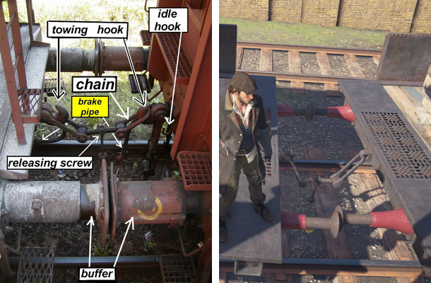
Fig. 1. On the left - details of the screw tie (source: Wikipedia [1]). On the right is the connective system in Assassin's Creed Syndicate.

In this case, our physical simulation gives a couple of advantages:

• Winding railway tracks are easier to control using a 1D simulator. Forcing 3D physics to use motion control limiters in a one-dimensional space is a rather risky decision. She can be very sensitive to the emerging instability, due to which the cars will take off into the air. However, we still needed to recognize the collisions of the cars in full 3D space.
• The moving connection provides more freedom in gameplay design. Compared to the real world, we need a much greater distance between the cars. This is required in order to have more space to perform different actions of the player and the camera (for example, to climb onto the roof of the car). In addition, our coupler is connected much less rigidly than in the real world to provide freer relative motion between the cars. This makes it easier for us to cope with sharp turns of railway tracks, and the recognition of collisions between cars protects against interpenetration.
• Thanks to our system, we can perform the uncoupling of cars (taking into account friction forces) and the calculation of collisions between uncoupled cars and the rest of the train (for example, when the train stops abruptly, when the uncoupled cars continue to move and as a result hit the train).

Here is a video with an example of the work of our physics:


We begin with a section in which we explain how trains are controlled.

Note: in order to simplify the explanation, we will designate the term “tractor” as a carriage closer to the locomotive, and the term “trailer” carriage that is located closer to the tail of the train.

Locomotive control

To control the locomotive, we have created a very simple interface consisting only of requests for the required speed:

Locomotive::SetDesiredSpeed(float DesiredSpeed, float TimeToReachDesiredSpeed) 

The rail system manager sends such requests for each train moving in the game. To fulfill the query, we calculate the force needed to create the required acceleration. We use the following formula (Newton's second law):



where F is the calculated force, m is the mass of the locomotive, (the required speed is the current speed), and t = TimeToReachDesiredSpeed ​​(time to reach the required speed) .

After calculating the force, we transfer it to WagonPhysicsState as the “engine power” to drive the locomotive (more on this in the next section).

Since the physical behavior of a train may depend, for example, on the number of cars (cars colliding with each other create a chain reaction and push the train forward), we need a way to ensure that the request sent to the desired speed is completely fulfilled. To achieve this, we re-compute the speed required to achieve the required speed every 2 seconds. Thus, we guarantee that the sent request will be executed as a result. But because of this, we cannot exactly match the value of TimeToReachDesiredSpeed . However, small time variations in the game are acceptable.

In addition, in order to maintain the locomotive speed specified by the SetDesiredSpeed request, we do not allow the coupling tie limiter to change the locomotive speed. To compensate for the absence of such impulses from limiters, we created a special method for simulating traction force (for more details, see the “Starting the train” section). And finally, we do not allow the reaction to collisions to change the speed of the locomotive, except for the case when the train brakes to zero speed.

The following section describes the basic level of physical simulation.

Basic simulation step

Here is the structure used to store physical information about each car (and locomotive):

 struct WagonPhysicsState { // ,   : //     . RailwayTrack m_Track; float m_LinearMomentum; // ,   . float m_LinearSpeed; //   . float m_EngineForce; float m_FrictionForce; //     ,    . Vector m_WorldPosition; Quaternion m_WorldRotation; //   : float m_Mass; } 

As you can see, the angular velocity is missing. Even if we check collisions between cars using 3D colliders (and the turn always corresponds to the direction of the tracks), trains move in a one-dimensional world along railway tracks. Therefore, for physics it is not necessary to store information about the angular motion. In addition, due to the one-dimensional simulation, for storing physical quantities (forces, impulses, and velocity), variables of type float are sufficient.

For each car, we use the Euler method [2] as the step of the basic simulation ( dt is the time of one simulation step):

 void WagonPhysicsState::BasicSimulationStep(float dt) { //  . float dPosition = m_LinearSpeed; float dLinearMomentum = m_EngineForce + m_FrictionForce; //  . m_LinearMomentum += dLinearMomentum*dt; m_LinearSpeed = m_LinearMomentum / m_Mass; //  . float DistanceToTravelDuringThisStep = dPosition*dt; m_Track.MoveAlongSpline( DistanceToTravelDuringThisStep ); //       . m_WorldPosition = m_Track.GetCurrentWorldPosition(); m_WorldRotation = m_Track.AlignToSpline(); } 

To implement BasicSimulationStep, we use three basic equations. These equations show that speed is a derivative of a position, and force is a derivative of a pulse (the point above the symbol denotes the derivative with respect to time) [2-4]:





In the third equation, the momentum P is determined, which is the product of mass and velocity:



In our implementation, applying a pulse to a car is simply a summation operation with the current pulse:

 void WagonPhysicsState::ApplyImpulse(float AmountOfImpulse) { m_LinearMomentum += AmountOfImpulse; m_LinearSpeed = m_LinearMomentum / m_Mass; } 

As you can see, immediately after the change in momentum, we recalculate the speed for more convenient access to this value. This is done in the same way as in [2].

Now, having a basic method of calculating changes over time, we can move on to other parts of the algorithm.

High-level simulation steps for one train

Here is the pseudo-code of the full simulation step for a single train:

 //       //       ApplyDeferredImpulses (  ) //       UpdateCouplingChainConstraint (   ) //       UpdateEngineAndFrictionForces (    ) SimulationStepWithFindCollision (    ) CollisionResponse (  ) 

It is important to mention that, as written in pseudocode, each part is performed sequentially for all the cars of one train. Part A implements a special behavior associated with the launch of the train. Part B applies pulses from collisions. Part B is a solution for an interconnect coupler, ensuring that we do not exceed the maximum distance for the interlock. Part G is responsible for engine power and friction, the basic simulation step (integration) and collision handling.

The simulation algorithm always preserves the same order of updates for train cars. We start with the locomotive and consistently go through all the cars of the train, from first to last. Since we can use this property in the simulator, it simplifies the formulation of calculations. We use this feature only for contact collisions, for sequential simulation of the movement of each car and checking the collision with only one neighboring car.

Each part of this high-level simulation cycle is discussed in detail in the following sections. Because of the special importance of part G, we will start with it and with SimulationStepWithFindCollision .

Collision simulation

Here is the code for the SimulationStepWithFindCollision function:

 WagonPhysicsState SimulationStepWithFindCollision(WagonPhysicsState InitialState, float dt) { WagonPhysicsState NewState = InitialState; NewState.BasicSimulationStep( dt ); bool IsCollision = IsCollisionWithWagonAheadOrBehind( NewState ); if (!IsCollision) { return NewState; } return FindCollision(InitialState, dt); } 

First, we perform a trial simulation step with a complete time change, causing

 NewState.BasicSimulationStep( dt ); 

and checking whether any collisions are detected in the new state:

 bool IsCollision = IsCollisionWithWagonAheadOrBehind( NewState ); 

If this method returns false , then the new computed state can be used directly. But if a collision is detected, we perform FindCollision to find a more accurate time and state of physics just before the collision event. To perform this task, we use a binary search similar to that used in [2].

Here is a cycle for finding a more accurate collision time and state of physics:

 WagonPhysicsState FindCollision(WagonPhysicsState CurrentPhysicsState, float TimeToSimulate) { WagonPhysicsState Result = CurrentPhysicsState; float MinTime = 0.0f; float MaxTime = TimeToSimulate; for (int step = 0 ; step<MAX_STEPS ; ++step) { float TestedTime = (MinTime + MaxTime) * 0.5f; WagonPhysicsState TestedPhysicsState = CurrentPhysicsState; TestedPhysicsState.BasicSimulationStep(TestedTime); if (IsCollisionWithWagonAheadOrBehind(TestedPhysicsState)) { MaxTime = TestedTime; } else { MinTime = TestedTime; Result = TestedPhysicsState; } } return Result; } 

Each iteration brings us closer to the exact time of the collision. We also know that it is necessary to check collisions with only one car, which is directly in front of the current car (or behind it, in case of reversal). To calculate the result, the IsCollisionWithWagonAheadOrBehind method uses collision checking between two oriented colliders (OBB). We check collisions in full 3D space using m_WorldPosition and m_WorldRotation from WagonPhysicsState .

Collision response

Having obtained the state of physics right before the collision event, we have to calculate the corresponding jet impulse j , in order to attach it to both the tractor and the trailer. We will start by calculating for the current relative speed between cars before a collision:



Similar relative speed after the collision event:



Where and - velocities after application of the impulse of reaction to collision j These velocities can be calculated using the pre-collision velocities and the momentum j as follows ( and - these are carriages masses):





Now we are ready to determine the coefficient of elastic recovery r :



The coefficient of elastic recovery determines how "elastic" the reaction to the collision. The value r = 0 means the total energy loss, the value r = 1 - the absence of energy loss (absolute elasticity). Substituting this equation into the previous formulas, we get





Order this equation to get momentum j :





Finally, we can calculate the momentum j :





In the game we use the coefficient of elastic recovery r = 0.35 .

We apply the impulse + j to the tractor and the impulse -j to the trailer. However, for the tractor we use “pending” impulses. Since we have already performed the integration for the tractor and do not want to change its current speed, we postpone the pulse to the next simulation frame. Visually, this is not very noticeable, because the difference in one frame is hardly visible. Such a “delayed” impulse is saved for the car and is used in part B of the next frame of the simulation.

Video with an example of a train stop:

Coupling tie

It is possible to perceive a connecting coupler as a limiter of the distance between the cars. To meet the requirement of this distance limiter, we calculate and apply the appropriate impulses to change speeds.

We start the calculation with the distance equation for the next simulation step. For every two cars connected by a coupler, we calculate the distances they will cover during the next simulation step. We can very easily calculate this distance using the current speed (and exploring integral equations):



where x is the distance, V is the current speed, and t is the time step of the simulation.

Then we calculate the formula:



Where:

- the distance that the tractor will travel at the next simulation step.

- the distance that the trailer will cover at the next simulation step.

If the FutureChainLength is greater than the maximum length of the connecting tie, then the distance limiter will be broken in the next simulation step. Accept that



If the distance limiter is broken, the value of d will be positive. In this case, in order to satisfy the condition of a distance limiter, we need to apply such impulses so that d = 0 . To establish the scale of the required impulses, use the weight of the car. It is necessary that the lighter car moves more, and the heavier one moves less. Assign the following factors and





Notice that . We need the trailer to go the extra distance in the next simulation step. , and the tractor - with a distance . To do this by applying a pulse, we need to multiply this distance by the mass divided by the time of the simulation step:





If you use the following additional coefficient C



then you can simplify impulse formulas to





You can see that they have the same size, but different signs.

After the application of both pulses, cars connected by such a coupling tie will not break the distance stop in the next simulation step. These pulses change speeds in such a way that as a result, in the integration formulas, positions are obtained that satisfy the condition of maximum distance for the tie.

However, even after calculating these pulses for one coupling tie, there is a possibility of breaking the maximum tie distance for other cars in the train. We will need to perform this method several times to reduce the final result. However, in practice it turned out that only one cycle is enough. It is enough to obtain satisfactory overall results.

We perform these calculations sequentially for each connecting tie in the train, starting with the locomotive. We always apply impulses to both cars connected by a coupler. But there is one exception to this rule: we never apply momentum to the locomotive. We need the locomotive to maintain its speed, so the impulse is applied only to the first carriage after the locomotive. This impulse is applied only to the trailer, which needs compensation for the entire required distance d (in this case we have , and ).

Correction during sharp turns

Since the simulation is carried out along a one-dimensional line, we have problems with perfect fit for the connecting tie on the hook when the cars move on sharp turns. In this situation, the 1D world intersects with the 3D world of the game. The connecting strap is located in the 3D world, but the impulses (compensating for satisfying the condition of the distance stop) are applied only in the simplified 1D world. To correct the determination of the final position of the tie on the hook, we slightly change the MaximumLengthOfCouplingChain depending on the relative angle between the directions of the tractor and the tie. The larger the angle, the shorter the maximum possible tie length. First, we compute the scalar product of two normalized vectors:



Where - the normalized direction of the connecting tie, and - vector of the forward direction of the tractor. Then we use the following formula to finally calculate the distance to be subtracted from the physical length of the connecting tie:

 float DistanceConvertedFromCosAngle = 2.0f*clamp( (1.0fs)-0.001f, 0.0f, 1.0f ); float DistanceSubtract = clamp( DistanceConvertedFromCosAngle, 0.0f, 0.9f ); 

As you can see, we do not calculate the exact value of the angle, but directly use the cosine. This saves us some computational time and this is enough for our needs. You can also use additional numbers based on empirical tests to limit the values ​​within acceptable limits. And finally, we use the DistanceSubtract value to satisfy the length limiter condition for the joint tie:

 MaximumLengthOfCouplingChain = ChainPhysicalLength - DistanceSubtract; 

It turned out that in practice these formulas work very well. They provide the correct hanging of the connecting tie on the hook, even on sharp turns in the route of the track.

Now we consider a special case - the start of the train.

Train start

As I mentioned earlier, we do not allow the impulses of the connecting tie to change the speed of the locomotive. However, we still need a way to simulate the effects of traction, especially when starting the train. When the locomotive starts, it starts to pull other cars, but the locomotive itself must also slow down according to the mass of the cars. To achieve this, we change speeds when the train accelerates from zero speed. We start with calculations based on the law of momentum balancing. This law states that “the impulse of the system is constant if external forces do not act on the system” [3]. This means that in our case the impulse before towing another car should be equal to the impulse Immediately after the tie strap pulls another car:





In our case, we can expand this to the following formula:



Where - weight of the i- th car ( - the mass of the locomotive), - the current speed of the locomotive (we assume that all already moving cars have the same speed as the locomotive), - system speed after towing (we assume that all towed cars have the same speed). If to use the additional designation defined as



then you can simplify the formula as follows



- this is the value we are looking for:



With this formula, you can simply set a new speed. for the locomotive and all cars (from 2 to n), which are currently pulled by a coupling coupler.
In Fig. 2 shows a schematic description of the pulse when the locomotive and two cars start to pull the third car :


Fig. 2. Start the train.

Here's a video of the train start:

Friction

To calculate the friction force (the m_FrictionForce variable in WagonPhysicsState ), the formulas and values ​​chosen after a series of experiments and most relevant to the gameplay are used. The value of the friction force is constant, but we additionally scale it according to the current speed (when the speed is below 4). Here is a graph of the standard friction force for wagons in the game:


Fig. 3. Standard friction force for wagons.

For disconnected cars other values ​​are used:


Fig. 4. Friction force for uncoupled wagons.

In addition, we wanted to give the player the ability to conveniently jump from car to car for a short period of time after disconnecting. Therefore, we used a lower friction value and scaled it relative to the time elapsed after the car was disconnected. The final friction value for uncoupled cars is set as follows:



where t is the time elapsed after the disconnect event (in seconds).

As you can see, we do not use friction for the first three seconds, and then gradually increase it.

Last notes

In game trains, we added moving bumpers in front and rear of the cars. These bumpers do not create any physical strength. We implemented their behavior as an additional visual element. They move according to the detected displacement of the adjacent bumper of another car.

In addition, as you can see, we do not check collisions between different trains in the simulator. The rail system manager is responsible for adjusting train speeds to avoid collisions. In our simulation, collisions are checked only between cars of the same train.

It is important to add that game sounds and special effects play a very important role in train perception. We compute various values ​​derived from physical behavior for controlling sounds and special effects (for example, the sounds of tightening a connecting tie, bumper bumps, braking, etc.).

Total

We talked about our physical train simulator, created for Assassin's Creed Syndicate. Working on this part of the game was a great pleasure and was very difficult.In the gameplay of the open world, there are many gameplay possibilities and various interactions. The open world creates even more difficulties in providing stable and sustainable systems. But after all the work done, it is very joyful to watch the trains moving in the game and contributing to the quality of the game process.

Thanks

I want to thank James Carnahan of Ubisoft Quebec City and Nobuyuki Miura of Ubisoft Singapore for editing this article and useful tips.

I also want to thank my colleagues from the Ubisoft Quebec City studio: Pierre Fortin, who helped me get started with train physics and inspired me to develop; Dave Tremblay for technical support; James Carnahan for all our talk of physics; Mathieu Pierrot (Matthieu Pierrot) for the inspiring approach; Maxim Begin, who was always ready to talk to me about programming; Vincent Martineau for his help. In addition, I am grateful to Martin Bedard (Marc Parenteau), Jonathan Gendron, Jonathan Gendron, Carl Dumont, Patrick Charland, Patrick Charland, Emil Uddestrand, Jéfélard (Patrick Charland), Emil Uddestrand, Em Jürden Dumont, Patrick Charland Damien Bastian), Eric Martel (Eric Martel), Steve Blezy (Steve Blezy), Patrick Legare (Patrick Legare),Guilherme Lupien, Eric Girard and everyone else who worked on Assassin's Creed Syndicate and created such an amazing game!

Reference materials

[1] “Buffers and chain coupler”, https://en.wikipedia.org/wiki/Buffers_and_chain_coupler [Approx. Per.: The Russian-language article on Wikipedia is rather superficial. Read more about the compounds used in the formulations here .]

[2] Andrew Witkin, David Baraff and Michael Kass, “An Introduction to Physical Based Modeling”, http://www.cs.cmu.edu/~baraff/pbm /

[3] Fletcher Dunn, Ian Parberry, “3D Math Primer for Graphics and Game Development, Second Edition”, CRC Press, Taylor & Francis Group, 2011.

[4] David H. Eberly, “Game Physics. Second Edition ”, Morgan Kaufmann, Elsevier, 2010.