Random Forest: walks in the winter forest

1. Introduction

This is a small practical guide to the use of machine learning algorithms. Of course, there is a considerable number of machine learning algorithms and methods of mathematical (statistical) analysis of information, however, this note is dedicated to Random Forest. The note shows examples of using this algorithm for problems of classification and regression, and also gives some theoretical explanations.

2. A few words about trees

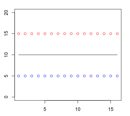
First of all, we will consider some basic theoretical principles of this algorithm, and let us begin with a concept such as decision trees. Our main task is to make a decision based on the available information. In the simplest case, we have only one sign (metric, predictor, regressor) with well distinguishable boundaries between classes (the maximum value for one class is clearly less than the minimum value for another). For example, knowing the body weight, it is necessary to distinguish a whale from a bee, if it is known that among all the observations there is not a single whale that has a body weight like that of a bee. Therefore, just one indicator (predictor) is enough to give an accurate answer, thus predicting the correct class.

Suppose that the points of one class (let them be shown in red) in all observations are above the blue points. A person can draw a straight line between them and say that this will be the border of classes. Therefore, everything located above this boundary will belong to one class, and everything below the line will belong to another.

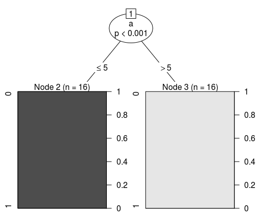
Let's display it in the form of a tree structure. If we use one of the algorithms (CART) to create a decision tree using the previously specified data, we get the following classification condition:

Conditional inference tree with 2 terminal nodes Response: class Input: a Number of observations: 32 1) a <= 5; criterion = 1, statistic = 31 2)* weights = 16 1) a > 5 3)* weights = 16 

Therefore, its visual presentation will be as follows:

Of course, each feature has a different degree of importance. From the following data set (LibSVM format) it is clear that the first sign (its index is 1, since the numbering does not start from zero) is absolutely identical in representatives of all classes. In fact, this indicator has no value for classification, therefore, it can be called redundant information that does not carry any practical benefits. The situation is similar with the second sign (predictor). However, the third one is different.

 1 1:10 2:20 3:4 0 1:10 2:20 3:5 1 1:10 2:20 3:4 0 1:10 2:20 3:5 1 1:10 2:20 3:4 0 1:10 2:20 3:5 1 1:10 2:20 3:4 0 1:10 2:20 3:5 1 1:10 2:20 3:4 0 1:10 2:20 3:5 

It is the third feature (feature 2) that will serve as the cherished distinction with which you can predict the class by vector. It is logical to assume that the problem can be solved by one single condition (If-Else). Indeed, each tree in the machine learning algorithm correctly understood the differences. The following shows debug information (using the Random Forest classifier from the Apache Spark 2.1.0 framework) for several trees of the random forest ensemble.

  Tree 0: If (feature 2 <= 4.0) Predict: 1.0 Else (feature 2 > 4.0) Predict: 0.0 Tree 1: If (feature 2 <= 4.0) Predict: 1.0 Else (feature 2 > 4.0) Predict: 0.0 Tree 2: If (feature 2 <= 4.0) Predict: 1.0 Else (feature 2 > 4.0) Predict: 0.0 

More complex tasks require more complex trees. In the following example, the pattern has ceased to be so obvious to humans. You need to look more closely at the dataset to notice the differences. The condition will be a bit more complicated, as additional verification is needed.

 1 1:10 2:25 0 1:10 2:20 1 1:15 2:20 0 1:10 2:20 1 1:10 2:25 0 1:10 2:20 1 1:15 2:20 0 1:10 2:20 1 1:10 2:25 0 1:10 2:20 1 1:15 2:20 0 1:10 2:20 

These additional checks require new branches (nodes) of the tree. After each branching, it will be necessary to do more checks, i.e. new branches. This can be seen on the debug information. In order to save space, I cite only a few trees:

  Tree 0: If (feature 0 <= 10.0) If (feature 1 <= 20.0) Predict: 0.0 Else (feature 1 > 20.0) Predict: 1.0 Else (feature 0 > 10.0) Predict: 1.0 Tree 1: If (feature 1 <= 20.0) If (feature 0 <= 10.0) Predict: 0.0 Else (feature 0 > 10.0) Predict: 1.0 Else (feature 1 > 20.0) Predict: 1.0 Tree 2: If (feature 1 <= 20.0) If (feature 0 <= 10.0) Predict: 0.0 Else (feature 0 > 10.0) Predict: 1.0 Else (feature 1 > 20.0) Predict: 1.0 

Now let's imagine a data set of a million rows and several hundred (even thousands) columns. Agree that with simple conditions such tasks will be difficult to solve. Moreover, under very difficult conditions (deep tree) it may be too specific for a particular data set (retrained). One tree is resistant to data scaling, but not to noise. If you combine a large number of trees in one composition, you can get much better results. The result is a very effective and fairly universal model.

3. Random Forest

In fact, Random Forest is a composition (ensemble) of many decision trees, which allows to reduce the problem of retraining and improve accuracy in comparison with a single tree. The forecast is obtained by aggregating the responses of multiple trees. The training of trees occurs independently of each other (on different subsets), which not only solves the problem of building identical trees on the same data set, but also makes this algorithm very convenient for use in distributed computing systems. In general, the idea of ​​bagging, proposed by Leo Braiman, is well suited for the distribution of calculations.

For bagging (independent learning of classification algorithms, where the result is determined by voting), it makes sense to use a large number of decision trees with a sufficiently large depth. During classification, the final result will be the class for which the majority of trees voted, provided that one tree has one vote.

For example, if a model with 500 trees was formed in the binary classification problem, among which 100 indicate the zero class, and the remaining 400 indicate the first class, then as a result the model will predict exactly the first class. If you use Random Forest for regression problems, then the approach of choosing the solution for which the majority of trees voted for would be inappropriate. Instead, there is a choice of the average solution for all trees.

Random Forest (due to the independent construction of deep trees) requires a lot of resources, and the limitation on depth will damage accuracy (to solve complex problems, you need to build many deep trees). It can be seen that the training time of trees increases approximately linearly in their number.

Naturally, an increase in the height (depth) of trees does not have the best effect on performance, but it increases the efficiency of this algorithm (although with this, the tendency to retraining increases). Too much fear of retraining should not be, as this will be compensated by the number of trees. But you shouldn't get carried away either. Everywhere, optimally matched parameters (hyperparameters) are important.

Consider an example of classification in the R programming language. Since we now need a classification model, rather than a regression model, the first parameter should be explicitly stated that the class is a factor. In addition to the number of trees, we will pay attention to the number of features (mtry) that the elementary model (tree) will use for branching. In fact, these are the two main parameters that it makes sense to configure in the first place.

 library(randomForest) dataset <- read.csv(file="/home/kalinin84/data/real.csv", head=TRUE, sep=",") model <- randomForest(factor(Class) ~ ., data=dataset, ntree=250, mtry=9) 

Make sure that this is exactly the model for classification:

 model$type 

Let's look at the confusion matrix results:

 model$confusion 

It is interesting to see the predicted values ​​(based on an out-of-bag):

 model$predicted 

And the varImpPlot and importance functions are intended for displaying the importance of predictors (values ​​for the accuracy of the classifier).

 varImpPlot(model) importance(model) 

Of course, there is a special function for obtaining a probable class. It is called predict. The model requires the first argument, and the data set as the second. The result will be a vector of predicted classes. For reliable testing, it is necessary to perform training on one data set, and check on another data set.

One more example. This time we use Apache Spark 2.1.0 and the Scala programming language. We read the information from a file of the LibSVM format. After that, it will be necessary to explicitly divide the data set into two parts. One of them will be educational, and the second - test. There is little point in standardizing or normalizing. Our model is resistant to this, as well as sufficiently resistant to data of different nature (weight, age, income).

I repeat that the training should be done only on the training sample. The number of classes in this example will be two. Let the number of trees be 50. Let's leave the Ginny index as a criterion for splitting, since theoretically the use of entropy would not be a much more effective criterion. The depth of the tree is limited to nine.

 import org.apache.spark.mllib.tree.RandomForest import org.apache.spark.mllib.tree.model.RandomForestModel import org.apache.spark.mllib.util.MLUtils val data = MLUtils.loadLibSVMFile(sc, "/home/kalinin84/data/real.data") val splits = data.randomSplit(Array(0.7, 0.3)) val (trainingData, testData) = (splits(0), splits(1)) val model = RandomForest.trainClassifier(trainingData, 2, Map[Int, Int](), 50, "auto", "gini", 9, 32) 

Now we use a test dataset to check the operation of the classifier with the specified parameters. It should be noted that the threshold of accuracy (suitability of the model) is determined individually in each specific case.

 import org.apache.spark.mllib.evaluation.BinaryClassificationMetrics val result = testData.map(p => (p.label, model.predict(p.features))) val metrics = new BinaryClassificationMetrics(result) // : 1.0 — ..    ROC metrics.areaUnderROC // : Array((0.0,0.0), (0.0,1.0), (1.0,1.0), (1.0,1.0)) metrics.roc.collect 

Having received the vector of predictors at the input, the system should guess (with an admissible probability) the class of the object. If, as a result of several checks on a large data set, this was done, then it is possible to assert the accuracy of the model. However, no person and no system will be able to guess with very high accuracy on the height of a person his level of education. Consequently, without properly collected and prepared data it will be difficult (or impossible at all) to solve the problem.

4. A few thoughts on practical application

There are such situations when a simple condition or methods of descriptive statistics cannot solve the problem right away. Just in the tasks of improving the efficiency of Internet projects (customer analysis, identifying purchase probability, optimal advertising strategies, selection of products for display in popular blocks, recommendations and personal rankings, classification of entries in catalogs and directories) and there are similar complex data sets.

I remember a few years ago I first encountered the need to use ML technologies. There was a situation when my colleagues (the development team) and I tried to come up with a method for classifying materials from a detailed reference on a very large portal. Previously, the classification was done manually by other specialists, which required a huge amount of time. But there was no way to automate (the rules and statistical methods did not give the required accuracy). We already had a set of vectors, which were previously marked out by experts.

Then I was surprised that several lines of code (using one of the popular machine learning libraries) were able to solve the problem almost immediately. Naturally, the possibility of using various models (including neural networks) was studied and rational hyperparameters were thought out. But since this note is about a random forest, the example in the Python programming language will be devoted to him. Naturally, the example code was written with regard to new versions of ready classifiers, and not used then:

 import pandas as pd from sklearn.metrics import classification_report, accuracy_score from sklearn.model_selection import train_test_split from sklearn.ensemble import RandomForestClassifier # #   # dataset = pd.read_csv('/home/kalinin84/data/real.csv') # #  (   ) # train, test = train_test_split(dataset, test_size = 0.4) classes = train.pop('Class').values features = train testClasses = test.pop('Class').values testFeatures = test # #   # model = RandomForestClassifier(n_estimators=500, max_depth=30).fit(features, classes) # #     # print(classification_report(testClasses, model.predict(testFeatures))) print(accuracy_score(testClasses, model.predict(testFeatures))) 

There are a lot of such examples. I'll tell you another story. The task was to increase the effectiveness of a huge advertising management system. Her work was directly dependent on the accuracy of predicting the rating of goods and services. Each of them had a vector of 64 signs. It was strategically important to give in advance a relatively accurate forecast of the value of the rating for each new feature vector. Prior to this, the system was governed by simple rules and descriptive statistics. But, as you know, efficiency and accuracy in such matters does not happen much. To solve the problem of increasing efficiency, a regression model was used, similar to that indicated in the example:

 from sklearn.datasets import load_svmlight_files from sklearn.metrics import mean_squared_error from sklearn.ensemble import RandomForestRegressor # #   (   ) # X, y, Xt, yt = load_svmlight_files(("/data/001.data", "/data/001_test.data")) # #        # model = RandomForestRegressor(n_estimators=500, max_features=5).fit(X,y) print(mean_squared_error(yt, model.predict(Xt))) # #        #        # import xgboost as xgb modelXGB = xgb.XGBRegressor().fit(X, y) print(mean_squared_error(yt, modelXGB.predict(Xt))) 

As a result, we get a fairly powerful tool for analyzing information that is able to come to the aid in those tasks where other methods do not give the best results.