Creating Hexagon Grid
Hexagonal meshes (hexagonal meshes) are used in some games, but they are not as simple and common as rectangle meshes. I have been collecting resources on hexagonal grids for almost 20 years, and I wrote this guide to the most elegant approaches implemented in the simplest code. The article often uses the manuals of Charles Fu ( Charles Fu ) and Clark Verbrugge. I will describe the different ways to create meshes of hexagons, their interconnection, as well as the most common algorithms. Many parts of this article are interactive: choosing a grid type changes the corresponding schemes, code, and texts. (Note. Lane: this applies only to the original, I advise you to study it. In translation, all the information of the original is stored, but without interactivity.) .
Code examples in the article are written in pseudocode, so they are easier to read and understand in order to write your own implementation.

Geometry
Hexagons are hexagonal polygons. In regular hexagons, all sides (faces) have the same length. We will work only with regular hexagons. Typically, horizontal (sharp-topped) and vertical (flat-topped) orientations are used in hexagonal meshes.
Hexagons with flat (left) and sharp (right) riding
')
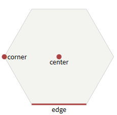
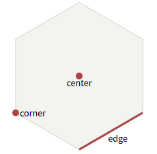
Hexagons have 6 faces. Each face is common to two hexagons. Hexagons have 6 corner points each. Each corner point is common to three hexagons. More information about centers, edges and corner points can be found in my article about the parts of grids (squares, hexagons and triangles).
Corners
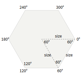
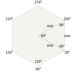
In a regular hexagon, the internal angles are 120 °. There are six “wedges”, each of which is an equilateral triangle with internal angles of 60 °. The corner point i is at a distance
(60° * i) + 30° , one size from the center . In the code: function hex_corner(center, size, i): var angle_deg = 60 * i + 30 var angle_rad = PI / 180 * angle_deg return Point(center.x + size * cos(angle_rad), center.y + size * sin(angle_rad)) To fill the hexagon, you need to get the vertices of the polygon with
hex_corner(…, 0) to hex_corner(…, 5) . To draw the outline of the hexagon, you need to use these vertices, and then draw the line again in hex_corner(…, 0) .The difference between the two orientations is that x and y change places, which leads to a change in angles: the angles of the hexagons with a flat top are 0 °, 60 °, 120 °, 180 °, 240 °, 300 °, and with a sharp top - 30 °, 90 °, 150 °, 210 °, 270 °, 330 °.
Angles of hexagons with flat and sharp top
Size and location
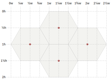
Now we want to arrange several hexagons together. In horizontal orientation, the height of the hexagon
height = size * 2 . Vertical distance between adjacent hexagons vert = height * 3/4 .Width of the hexagon
width = sqrt(3)/2 * height . Horizontal distance between adjacent hexagons horiz = width .In some games, pixel art is used for hexagons, which does not exactly correspond to regular hexagons. The formulas of angles and arrangements described in this section will not coincide with the size of such hexagons. The rest of the article, describing the algorithms of the grids of hexagons, is applicable even if the hexagons are slightly stretched or compressed.

Coordinate systems
Let's start assembling hexagons into a grid. In the case of square grids, there is only one obvious way to assemble. For hexagons, there are many approaches. I recommend using cubic coordinates as the primary representation. Axial or offset coordinates should be used to store maps and display coordinates for the user.
Offset Coordinates
The most common approach is to offset each successive column or row. Columns are denoted by
col or q . Rows are designated row or r . You can offset odd or even columns / rows, so horizontal and vertical hexagons have two options.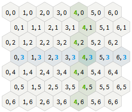
Horizontal arrangement "odd-r"

Horizontal arrangement "even-r"
Vertical arrangement "odd-q"
Vertical arrangement "even-q"
Cubic coordinates
Another way to consider the grids of hexagons is to see three main axes in them, rather than two , as in the grids of squares. They show elegant symmetry.
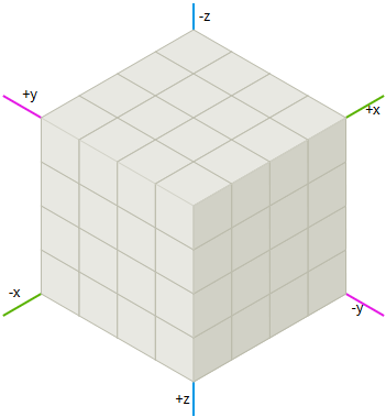
Take a grid of cubes and cut a diagonal plane at
x + y + z = 0 . This is a strange thought, but it will help us to simplify the algorithms of the grids of hexagons. In particular, we will be able to use standard operations from Cartesian coordinates: summation and subtraction of coordinates, multiplication and division by a scalar quantity, as well as distances.Notice the three major axes on the grid of cubes and their relationship to the six diagonal directions of the grid of hexagons. The diagonal axes of the grid correspond to the main direction of the grid of hexagons.
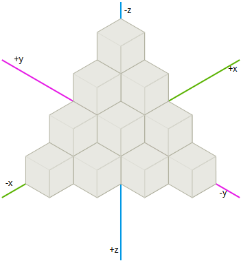
Hexagons
Cubes
Since we already have algorithms for grids of squares and cubes, the use of cubic coordinates allows us to adapt these algorithms to the grid of hexagons. I will use this system for most article algorithms. To use algorithms with a different coordinate system, I will transform the cubic coordinates, execute the algorithm, and then transform them back.
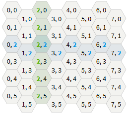
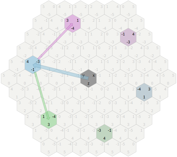
Learn how cubic coordinates work for a grid of hexagons. When selecting hexagons, the cubic coordinates corresponding to the three axes are highlighted.
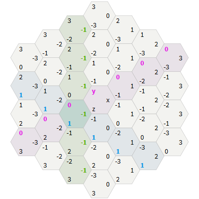
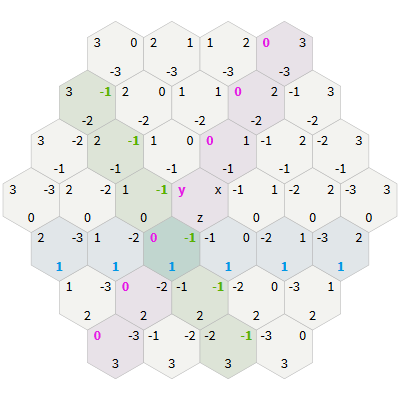
- Each direction of the grid of cubes corresponds to a line on the grid of hexagons. Try selecting a hexagon with
zequal to 0, 1, 2, 3 to see the connection. The line is marked in blue. Try the same forx(green) andy(lilac). - Each direction of the hexagon grid is a combination of two directions of the grid of cubes. For example, the "north" of the grid of hexagons lies between
+yand-z, so each step to the "north" increasesyby 1 and decreaseszby 1.
Cubic coordinates are a reasonable choice for a coordinate system of a grid of hexagons. The condition is
x + y + z = 0 , so it must be preserved in the algorithms. The condition also ensures that for each hexagon there will always be a canonical coordinate.There are many different coordinate systems for cubes and hexagons. In some of them, the condition is different from
x + y + z = 0 . I showed only one of many systems. You can also create cubic coordinates with xy , yz , zx , which will have their own set of interesting properties, but I will not consider them here.But you can argue that you do not want to store 3 numbers for the coordinates, because you do not know how to store the map in this form.
Axial coordinates
An axial coordinate system, sometimes referred to as “trapezoidal,” is constructed on the basis of two or three coordinates from a cubic coordinate system. Since we have the condition
x + y + z = 0 , the third coordinate is not needed. Axial coordinates are useful for storing maps and displaying coordinates to the user. As in the case of cubic coordinates, standard summation, subtraction, multiplication, and division of Cartesian coordinates can be used with them.There are many cubic coordinate systems and many axial. In this guide, I will not consider all combinations. I will select two variables,
q (column) and r (string). In the schemes of this article, q corresponds to x , and r corresponds to z , but such a correspondence is arbitrary, because it is possible to rotate and rotate the schemes, obtaining various correspondences.The advantage of this system over offsets offsets is the greater clarity of the algorithms. The disadvantage of the system is that storing a rectangular card is a bit strange; See the section on saving maps. Some algorithms are even clearer in cubic coordinates, but since we have the condition
x + y + z = 0 , we can calculate the third implied coordinate and use it in these algorithms. In my projects, I call the q , r , s axes, so the condition looks like q + r + s = 0 , and I can calculate s = -q - r when needed.Axles
The offset coordinates are the first things that most people think about, because they coincide with the standard Cartesian coordinates used for square grids. Unfortunately, one of the two axles must pass “against the fur,” and this makes it all the more difficult. The cubic and axial systems go "on the fur" and they have simpler algorithms, but storing maps is a bit more complicated. There is another system called “interlaced” or “double”, but here we will not consider it; some believe that it is easier to work with it than with a cubic or axial one.
Offset coordinates, cubic and axial
The axis is the direction in which the corresponding coordinate increases. The perpendicular to the axis is the line on which the coordinate remains constant. The grid diagrams above show perpendicular lines.
Coordinate Transformation
It is likely that you will use axial coordinates or displacement coordinates in your project, but many algorithms are easier expressed in cubic coordinates. Therefore, we need to be able to convert coordinates between systems.
The axial coordinates are closely related to cubic ones, so the conversion is simple:
# q = x r = z # x = q z = r y = -xz In code, these two functions can be written as follows:
function cube_to_hex(h): # var q = hx var r = hz return Hex(q, r) function hex_to_cube(h): # var x = hq var z = hr var y = -xz return Cube(x, y, z) The offset coordinates are quite a bit more complicated:
# -q col = x row = z + (x + (x&1)) / 2 # -q x = col z = row - (col + (col&1)) / 2 y = -xz # -q col = x row = z + (x - (x&1)) / 2 # -q x = col z = row - (col - (col&1)) / 2 y = -xz # -r col = x + (z + (z&1)) / 2 row = z # -r x = col - (row + (row&1)) / 2 z = row y = -xz # -r col = x + (z - (z&1)) / 2 row = z # -r x = col - (row - (row&1)) / 2 z = row y = -xz Implementation note: I use a & 1 ( bitwise "AND" ) instead of a% 2 ( division with remainder ) to determine whether the number is even (0) or odd (1). For a detailed description, see the notes page for my implementation .
Neighboring Hexagons
Given one hexagon, with which six hexagons is it adjacent? As you might expect, the easiest way to answer is in cubic coordinates, quite simple in axial coordinates, and a bit more difficult in offset coordinates. You may also need to calculate six "diagonal" hexagons.
Cubic coordinates
Moving one space in the coordinates of the hexagons leads to a change in one of the three cubic coordinates by +1 and the other by -1 (the sum must remain 0). Three possible coordinates can be changed by +1, and the remaining two can be changed by -1. This gives us six possible changes. Each corresponds to one of the directions of the hexagon. The simplest and fastest way is to precompute the changes and put them into the table of
Cube(dx, dy, dz) cubic coordinates during compilation: var directions = [ Cube(+1, -1, 0), Cube(+1, 0, -1), Cube( 0, +1, -1), Cube(-1, +1, 0), Cube(-1, 0, +1), Cube( 0, -1, +1) ] function cube_direction(direction): return directions[direction] function cube_neighbor(hex, direction): return cube_add(hex, cube_direction(direction)) 
Axial coordinates
As before, we use a cubic system to begin with. Take the
Cube(dx, dy, dz) table Cube(dx, dy, dz) and convert to the Hex(dq, dr) table Hex(dq, dr) : var directions = [ Hex(+1, 0), Hex(+1, -1), Hex( 0, -1), Hex(-1, 0), Hex(-1, +1), Hex( 0, +1) ] function hex_direction(direction): return directions[direction] function hex_neighbor(hex, direction): var dir = hex_direction(direction) return Hex(hex.q + dir.q, hex.r + dir.r) 
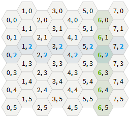
Offset coordinates
In axial coordinates, we make changes depending on where in the grid we are. If we are in an offset column / row, then the rule is different from the case of a column / row without offset.
As before, we create a table of numbers that need to be added to
col and row . However, this time we will have two arrays, one for odd columns / rows, and the other for even ones. Look at (1,1) in the figure above for the grid map and notice how col and row change when moving in each of the six directions. Now repeat the process for (2,2) . The tables and the code will be different for each of the four types of offset grids; we give the corresponding code for each type of grid.Odd-r
var directions = [ [ Hex(+1, 0), Hex( 0, -1), Hex(-1, -1), Hex(-1, 0), Hex(-1, +1), Hex( 0, +1) ], [ Hex(+1, 0), Hex(+1, -1), Hex( 0, -1), Hex(-1, 0), Hex( 0, +1), Hex(+1, +1) ] ] function offset_neighbor(hex, direction): var parity = hex.row & 1 var dir = directions[parity][direction] return Hex(hex.col + dir.col, hex.row + dir.row) 
Grid for even (EVEN) and odd (ODD) rows
Even-r
var directions = [ [ Hex(+1, 0), Hex(+1, -1), Hex( 0, -1), Hex(-1, 0), Hex( 0, +1), Hex(+1, +1) ], [ Hex(+1, 0), Hex( 0, -1), Hex(-1, -1), Hex(-1, 0), Hex(-1, +1), Hex( 0, +1) ] ] function offset_neighbor(hex, direction): var parity = hex.row & 1 var dir = directions[parity][direction] return Hex(hex.col + dir.col, hex.row + dir.row) 
Grid for even (EVEN) and odd (ODD) rows
Odd-q
var directions = [ [ Hex(+1, 0), Hex(+1, -1), Hex( 0, -1), Hex(-1, -1), Hex(-1, 0), Hex( 0, +1) ], [ Hex(+1, +1), Hex(+1, 0), Hex( 0, -1), Hex(-1, 0), Hex(-1, +1), Hex( 0, +1) ] ] function offset_neighbor(hex, direction): var parity = hex.col & 1 var dir = directions[parity][direction] return Hex(hex.col + dir.col, hex.row + dir.row) 
Grid for even (EVEN) and odd (ODD) columns
Even-q
var directions = [ [ Hex(+1, +1), Hex(+1, 0), Hex( 0, -1), Hex(-1, 0), Hex(-1, +1), Hex( 0, +1) ], [ Hex(+1, 0), Hex(+1, -1), Hex( 0, -1), Hex(-1, -1), Hex(-1, 0), Hex( 0, +1) ] ] function offset_neighbor(hex, direction): var parity = hex.col & 1 var dir = directions[parity][direction] return Hex(hex.col + dir.col, hex.row + dir.row) 
Grid for even (EVEN) and odd (ODD) columns
Using the above lookup tables is the easiest way to calculate neighbors. If you're interested, you can also read about extracting these numbers .
Diagonals
The displacement in the “diagonal” space in the coordinates of the hexagons changes one of the three cubic coordinates by ± 2 and the other two by ∓1 (the sum must remain equal to 0).
var diagonals = [ Cube(+2, -1, -1), Cube(+1, +1, -2), Cube(-1, +2, -1), Cube(-2, +1, +1), Cube(-1, -1, +2), Cube(+1, -2, +1) ] function cube_diagonal_neighbor(hex, direction): return cube_add(hex, diagonals[direction]) As before, we can convert these coordinates into axial ones, by folding one of the three coordinates, or convert them into offset coordinates, having previously calculated the results.

Distances
Cubic coordinates
In a cubic coordinate system, each hexagon is a cube in three-dimensional space. Neighboring hexagons are in a grid of hexagons at a distance of 1 from each other, but at a distance of 2 in a grid of cubes. This makes distance calculation simple. In the grid of squares, the Manhattan distances are equal to
abs(dx) + abs(dy) . In a grid of cubes, the Manhattan distances are equal to abs(dx) + abs(dy) + abs(dz) . The distance in the grid of hexagons is half of them: function cube_distance(a, b): return (abs(ax - bx) + abs(ay - by) + abs(az - bz)) / 2 The equivalent of this record will be the expression that one of the three coordinates should be the sum of the other two, and then get it as a distance. You can choose the form of division in half or the form of the maximum value given below, but they give the same result:
function cube_distance(a, b): return max(abs(ax - bx), abs(ay - by), abs(az - bz)) In the figure, the maximum values are highlighted in color. Notice also that each color represents one of the six "diagonal" directions.
Gif
Axial coordinates
In the axial system, the third coordinate is implicitly expressed. Let's convert from an axial to a cubic system to calculate the distance:
function hex_distance(a, b): var ac = hex_to_cube(a) var bc = hex_to_cube(b) return cube_distance(ac, bc) If the compiler in your case embeds (inline)
hex_to_cube and cube_distance , then it will generate the following code: function hex_distance(a, b): return (abs(aq - bq) + abs(aq + ar - bq - br) + abs(ar - br)) / 2 There are many different ways to record the distances between the hexagons in axial coordinates, but regardless of the recording method, the distance between the hexagons in the axial system is extracted from the Manhattan distance in the cubic system . For example, the “difference of differences” described here is obtained from the record
aq + ar - bq - br as aq - bq + ar - br and using the maximum value form instead of the halving cube_distance . All of them are similar, if you see the connection with cubic coordinates.Offset coordinates
As in the case of axial coordinates, we convert the displacement coordinates into cubic coordinates, and then use the distance of the cubic system.
function offset_distance(a, b): var ac = offset_to_cube(a) var bc = offset_to_cube(b) return cube_distance(ac, bc) We will use the same pattern for many algorithms: convert from hexagons to cubes, execute the cubic version of the algorithm, and convert the cubic results into hexagon coordinates (axial or displacement coordinates).
Line drawing
How to draw a line from one hexagon to another? I use linear interpolation to draw lines . The line is uniformly sampled at
N+1 points and it is calculated in which hexagons these samples are located.Gif
- First we calculate
N, which will be the distance in the hexagons between the end points. - Then we uniformly sample
N+1points between points A and B. Using linear interpolation, we determine that forivalues from0toN, including them, each point will beA + (B - A) * 1.0/N * i. In the figure, these control points are shown in blue. As a result, floating point coordinates are obtained. - Transform each control point (float) back into hexagons (int). The algorithm is called
cube_round(see below).
We put everything together to draw the line from A to B:
function lerp(a, b, t): // float return a + (b - a) * t function cube_lerp(a, b, t): // return Cube(lerp(ax, bx, t), lerp(ay, by, t), lerp(az, bz, t)) function cube_linedraw(a, b): var N = cube_distance(a, b) var results = [] for each 0 ≤ i ≤ N: results.append(cube_round(cube_lerp(a, b, 1.0/N * i))) return results Notes:
- There are cases when
cube_lerpreturns a point exactly on the edge between two hexagons. Thencube_roundshifts it in one direction or another. Lines look better if they are shifted in one direction. This can be done by adding an "epsilon" hexagonalCube(1e-6, 1e-6, -2e-6)to one or both end points before the start of the cycle. This “pushes” the line in one direction so that it does not fall on the edges of the faces. - The DDA line algorithm in grid squares equates
Nwith the maximum distance along each of the axes. We do the same in cubic space, which is similar to the distance in the grid of hexagons. - The
cube_lerpfunction should return a cube with coordinates in float. If you are programming in a language with static typing, you will not be able to use theCubetype. Instead, you can define the typeFloatCubeor embed (inline) the function in the line drawing code, if you do not want to define another type. - You can optimize the code by inserting (inline)
cube_lerp, and then calculatingBx-Ax,Bx-Ayand1.0/Noutside the loop. Multiplication can be converted to repeated summation. The result is something like a DDA-line algorithm. - To draw lines, I use axial or cubic coordinates, but if you want to work with offset coordinates, then read this article .
- There are many options for drawing lines. Sometimes a "supercover" is required. They sent me a code for drawing lines with overcoating in hexagons, but I have not studied it yet.
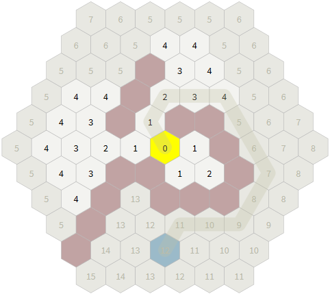
Movement range
Coordinate Range
For a given center of a hexagon and a range of
N which hexagons are located within N steps from it?We can do the reverse work from the distance between hexagons formula
distance = max(abs(dx), abs(dy), abs(dz)) . To find all hexagons within N , we need max(abs(dx), abs(dy), abs(dz)) ≤ N This means that we need all three values: abs(dx) ≤ N and abs(dy) ≤ N and abs(dz) ≤ N Removing the absolute value, we get -N ≤ dx ≤ N and -N ≤ dy ≤ N and -N ≤ dz ≤ N In the code, this will be a nested loop: var results = [] for each -N ≤ dx ≤ N: for each -N ≤ dy ≤ N: for each -N ≤ dz ≤ N: if dx + dy + dz = 0: results.append(cube_add(center, Cube(dx, dy, dz))) This cycle will work, but will be rather ineffective. Of all the
dz values that we loop through, only one really satisfies the cubes condition dx + dy + dz = 0 . Instead, we directly calculate the value of dz satisfying the condition: var results = [] for each -N ≤ dx ≤ N: for each max(-N, -dx-N) ≤ dy ≤ min(N, -dx+N): var dz = -dx-dy results.append(cube_add(center, Cube(dx, dy, dz))) This cycle takes place only at the desired coordinates. In the figure, each range is a pair of lines. Each line is an inequality. We take all hexagons satisfying six inequalities.
Gif
Intersecting ranges
If you need to find hexagons that are in several ranges, then before generating a list of hexagons, you can cross ranges.
One can approach this problem from the point of view of algebra or geometry. Algebraically, each domain is expressed as conditions of inequalities in form
-N ≤ dx ≤ N, and we need to find the intersection of these conditions. Geometrically, each region is a cube in three-dimensional space, and we will intersect two cubes in three-dimensional space to obtain a rectangular parallelepiped in three-dimensional space. Then we project it back onto the plane x + y + z = 0to get the hexagons. I will solve this problem algebraically.First, we rewrite the condition
-N ≤ dx ≤ Nin a more general form , and accept and . Do the same forx min ≤ x ≤ x maxx min = center.x - Nx max = center.x + Nyand z, as a result, getting a general view of the code from the previous section: var results = [] for each xmin ≤ x ≤ xmax: for each max(ymin, -x-zmax) ≤ y ≤ min(ymax, -x-zmin): var z = -xy results.append(Cube(x, y, z)) The intersection of two ranges
a ≤ x ≤ band c ≤ x ≤ dis max(a, c) ≤ x ≤ min(b, d). Because the area of the hexagons expressed as ranges of x, y, zwe can individually to cross each of the bands x, y, zand then use a nested loop to generate a list of the hexagons in an intersection. For one area of hexagons we accept and , similarly for and . To intersect two regions of hexagons, we take and max = min (H1.x + N, H2.x + N), similarly for and . The same pattern works for intersecting three or more areas.x min = Hx - Nx max = Hx + Nyzx min = max(H1.x - N, H2.x - N)xyzGif
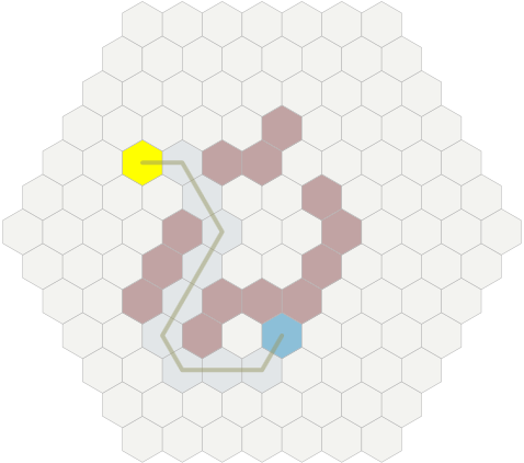
Obstacles
If there are obstacles, the easiest way to do this is to fill with a distance restriction (wide search). In the figure below we are limited to four moves. In code
fringes[k], this is an array of all hexagons that can be reached in ksteps. With each pass through the main loop, we expand the level k-1to the level k. function cube_reachable(start, movement): var visited = set() add start to visited var fringes = [] fringes.append([start]) for each 1 < k ≤ movement: fringes.append([]) for each cube in fringes[k-1]: for each 0 ≤ dir < 6: var neighbor = cube_neighbor(cube, dir) if neighbor not in visited, not blocked: add neighbor to visited fringes[k].append(neighbor) return visited Turns
For a given hexagon vector (the difference between two hexagons) we may need to rotate it so that it points to another hexagon. This is easy to do, having cubic coordinates, if you stick to a turn by 1/6 of a circle.
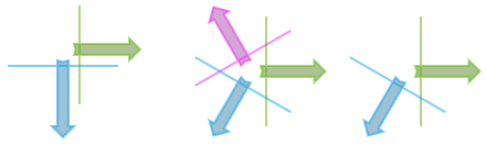
Rotate 60 ° to the right shifts each coordinate one position to the right:
[ x, y, z] to [-z, -x, -y] Rotate 60 ° to the left shifts each coordinate one position to the left:
[ x, y, z] to [-y, -z, -x] 
“Having played” [in the original of the article] with the scheme, one can notice that each turn by 60 ° changes signs and physically “rotates” the coordinates. After turning to 120 °, the signs again become the same. A 180 ° rotation changes signs, but the coordinates rotate to their original position.
Here is the complete sequence of turning the position P around the center position C, leading to the new position R:
- Transformation of P and C positions into cubic coordinates.
- Center vector calculation by subtracting:
P_from_C = P - C = Cube(Px - Cx, Py - Cy, Pz - Cz). - Rotate the vector
P_from_Cas described above and assign the notation to the final vectorR_from_C. - Transformation vectors back into the center position of addition:
R = R_from_C + C = Cube(R_from_C.x + Cx, R_from_C.y + Cy, R_from_C.z + Cz). - Convert the cubic position of R back to the desired coordinate system.
There are several stages of transformation, but each one is fairly simple. You can shorten some of these steps by defining the rotation directly in the axial coordinates, but the hexagon vectors do not work with the offset coordinates, and I do not know how to shorten the steps for the offset coordinates. See also the discussion of other ways to calculate rotation on stackexchange.
Rings
Simple ring
To find out if a given hexagon belongs to a ring of a given radius
radius, you need to calculate the distance from this hexagon to the center, and find out if it is equal radius. To get a list of all such hexagons, you need to take radiussteps from the center, and then follow the turning vectors along the path along the ring. function cube_ring(center, radius): var results = [] # radius == 0; , ? var cube = cube_add(center, cube_scale(cube_direction(4), radius)) for each 0 ≤ i < 6: for each 0 ≤ j < radius: results.append(cube) cube = cube_neighbor(cube, i) return results This code
cubestarts on a ring, shown by a large arrow from the center to the corner of the circuit. I chose angle 4 to begin with, because it corresponds to the path in which my numbers of directions move. You may need a different starting angle. At each stage of the internal cycle cubemoves one hexagon around the ring. Through the 6 * radiussteps he completes where he started.

Spiral rings
Passing through the rings in a spiral pattern, we can fill the inner parts of the rings:
function cube_spiral(center, radius): var results = [center] for each 1 ≤ k ≤ radius: results = results + cube_ring(center, k) return results 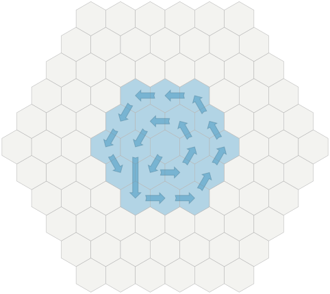

The area of the large hexagon is equal to the sum of all circles plus 1 for the center. To calculate the area, use this formula .
Traversing hexagons in this way can also be used to calculate the range of motion (see above).
Area of visibility
What is visible from a given position with a given distance, and does not overlap with obstacles? The simplest way to determine this is to draw a line to each hexagon in a given range. If the line does not meet with the walls, then you see a hexagon. Move the mouse over the hexagons [on the diagram in the original article] to see the lines drawn to these hexagons and the walls with which the lines meet.
This algorithm can be slow on large areas, but it is easy to implement, so I recommend starting with it.
Gif
There are many different definitions of visibility. Do you want to see the center of another hexagon from the center of the initial one? Do you want to see any part of the other hexagon from the center of the initial one? Maybe any part of another hexagon from anywhere in the starting one? Obstacles that hinder the view are smaller than a full hexagon? Scope is a trickier and more diverse concept than it seems at first glance. Let's start with the simplest algorithm, but expect that it will correctly calculate the answer in your project. There are even cases when a simple algorithm gives illogical results.
The Clark Verbrugge manual describes an algorithm for calculating the "start from the center of scope" and move outward. " See also the Duelo project , which is on Github.online demo scope with directions . You can also read my article on the calculation of 2d visibility , it has an algorithm that works with polygons, including hexagons. The roguelike community has a good set of algorithms for squares grids (see here , here and here). Some of them can be adapted to the grid of hexagons.
Hexagons to pixels
To convert from hexagons to pixels, it is useful to study the size and location scheme presented in the Geometry section. In the case of axial coordinates, the transformation from hexagons to pixels must be approached, considering the basis vectors. In the diagram, the arrow A → Q is the basis vector q, and A → R is the basis vector r. The pixel coordinate is
q_basis * q + r_basis * r. For example, B in (1, 1) is the sum of the basis vectors q and r.
In the presence of a matrix library, the operation is a simple multiplication of matrices. However, here I will write the code without matrices. For an axial grid
x = q, z = rwhich I use in this guide, the transformation will be as follows:For flat-topped hexagons
function hex_to_pixel(hex): x = size * 3/2 * hex.q y = size * sqrt(3) * (hex.r + hex.q/2) return Point(x, y) For hexagons with sharp tops
function hex_to_pixel(hex): x = size * sqrt(3) * (hex.q + hex.r/2) y = size * 3/2 * hex.r return Point(x, y) The matrix approach will be convenient later when we need to convert the coordinates of the pixels back to the coordinates of the hexagons. All we need is to invert the matrix. For cubic coordinates, you can either use cubic basis vectors (x, y, z), or first convert them to axial, and then use axial basis vectors (q, r).
For offset coordinates, we will need to shift the number of the column or row (it will no longer be an integer). After that, you can use the basic vectors q and r associated with the x and y axes:
Odd-r
function offset_to_pixel(hex): x = size * sqrt(3) * (hex.col + 0.5 * (hex.row&1)) y = size * 3/2 * hex.row return Point(x, y) Even-r
function offset_to_pixel(hex): x = size * sqrt(3) * (hex.col - 0.5 * (hex.row&1)) y = size * 3/2 * hex.row return Point(x, y) Odd-q
function offset_to_pixel(hex): x = size * 3/2 * hex.col y = size * sqrt(3) * (hex.row + 0.5 * (hex.col&1)) return Point(x, y) Even-q
function offset_to_pixel(hex): x = size * 3/2 * hex.col y = size * sqrt(3) * (hex.row - 0.5 * (hex.col&1)) return Point(x, y) Unfortunately, the offset coordinates do not have basis vectors that can be used with the matrix. This is one of the reasons why converting from pixels to hexagons is more difficult in offset coordinates.
Another approach is to convert the offset coordinates to cubic / axial coordinates, then use the conversion of cubic / axial coordinates to pixels. By embedding the transform code while optimizing it, it will result in the same result as above.
From pixels to hexagons
One of the most frequent questions is how to take the position of a pixel (for example, a mouse click) and convert it to the coordinate of the grid of hexagons? I will show how this is done for axial or cubic coordinates. For offset coordinates, the easiest way is to convert cubic coordinates to offset coordinates at the end.
Gif
- First we invert the hexagon transformation to pixels. This will give us the fractional coordinates of the hexagon, shown in the picture with a small blue circle.
- Then we define a hexagon containing the fractional coordinate of the hexagon. It is shown in the figure by a highlighted hexagon.
For the coordinate conversion in the pixel coordinates of hexagons we have multiplied
q, rthe basis vectors to obtain x, y. It can be considered a multiplication of matrices. Here is a matrix for hexagons with sharp tops: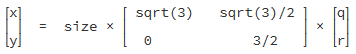
Converting pixel coordinates back to hexagon coordinates is fairly straightforward. We can reverse the matrix:

These calculations will give us fractional axial coordinates (float) for
qand r. The function hex_round()converts fractional axial coordinates to whole axial coordinates of hexagons.Here is the code for axial hexagons with sharp tops:
function pixel_to_hex(x, y): q = (x * sqrt(3)/3 - y / 3) / size r = y * 2/3 / size return hex_round(Hex(q, r)) And here is the code for axial hexagons with flat tops:
function pixel_to_hex(x, y): q = x * 2/3 / size r = (-x / 3 + sqrt(3)/3 * y) / size return hex_round(Hex(q, r)) These three lines of code transform the pixel position into the axial coordinate of the hexagon. If you use offset coordinates, then use
return cube_to_hex(cube_round(Cube(q, -qr, r))).There are many other ways to convert pixels to hexagons. On this page are the known to me.
Round to nearest hexagon
Sometimes we get a cubic coordinate (x, y, z) with a floating point , and we need to know in which hexagon it should be. This turns out to be a line drawing and a conversion from pixels to hexagons. Converting a floating point value to an integer value is called rounding , so I called this algorithm
cube_round.In cubic coordinates,
x + y + z = 0even with cubic floating point coordinates. So let's round each component down to the nearest integer (rx, ry, rz). However, although x + y + z = 0, after rounding, we have no guarantees that rx + ry + rz = 0. Therefore, we change the component with the largest change so that the condition is rx + ry + rz = 0true. For example, if the change is y abs(ry-y)greaterabs(rx-x)and abs(rz-z), then we change it to ry = -rx-rz. This guarantees us that rx + ry + rz = 0. Here is the algorithm: function cube_round(h): var rx = round(hx) var ry = round(hy) var rz = round(hz) var x_diff = abs(rx - hx) var y_diff = abs(ry - hy) var z_diff = abs(rz - hz) if x_diff > y_diff and x_diff > z_diff: rx = -ry-rz else if y_diff > z_diff: ry = -rx-rz else: rz = -rx-ry return Cube(rx, ry, rz) For non-cubic coordinates, the easiest way is to convert them to cubic coordinates, use the rounding algorithm, and then convert them back:
function hex_round(h): return cube_to_hex(cube_round(hex_to_cube(h))) Implementation note:
cube_roundand hex_roundget the coordinates in float, not in int. If you have written classes Cubeand Hex, they will work fine in languages with dynamic typing, in which you can pass floating-point numbers instead of integers, and in languages with static typing with a unified type of numbers. However, in most languages with static typing, a separate class / struct type for float coordinates cube_roundwill be needed and will be of type FloatCube → Cube. If you also need it hex_round, it will be FloatHex → Hexusing a helper function floatcube_to_floathexinstead cube_to_hex. In languages with parameterized types (C ++, Haskell, etc.), you can define a Cube, where T is an int or float. Or you can writecube_round to get three floating point numbers as input instead of defining a new type only for this function.Storage of maps in axial coordinates
Most often, the axial coordinate system causes complaints because it leads to unnecessary expenditure of space when using rectangular maps. This is one of the reasons in favor of the offset coordinate system. However, all the coordinate systems of hexagons lead to the consumption of space when using triangular or hexagonal maps. We can use the same strategy for storing all these types of cards.

Rectangular Map

Triangular Map

Hexagon Map
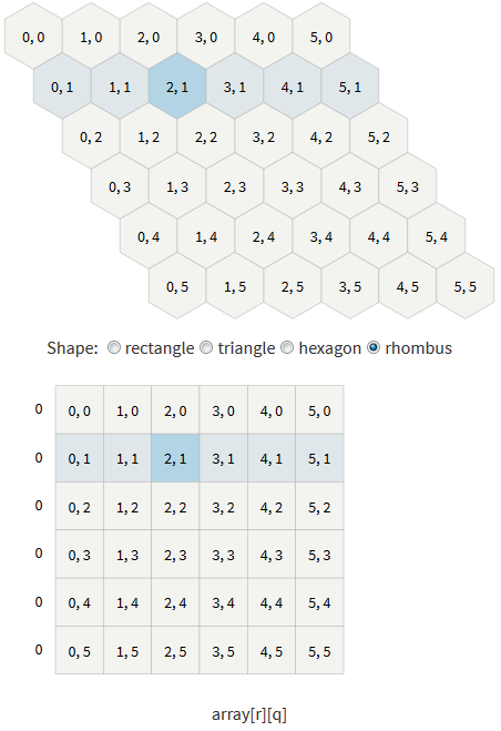
Diamond Card
Notice in the diagram that the unused space is to the right and left of each line (except for diamond-shaped cards). This gives us three options for card storage strategies:
- . . . , .
- - . , .
q,rhash_table(hash(q,r)). / , . - . . . . , 0, .
, « ».q,r,array[r][q - first_column[r]]. / , .first_column.
, « » « », .first_column[r] == -floor(r/2).array[r][q + r/2], .- , ,
first_column[r] == 0,access array[r][q]— ! , - ( ),array[r][q+r]. N,N = max(abs(x), abs(y), abs(z),first_column[r] == -N - min(0, r).array[r][q + N + min(0, r)]. -r < 0,array[r + N][q + N + min(0, r)].- ,
array[r][q].
Some games require the card to “stick together” along the edges. A square map can be wrapped only along the x axis (which roughly corresponds to a sphere) or along both x and y axes (which roughly corresponds to a torus). Folding depends on the shape of the map, and not on the shape of its elements. Folding a square map is easier done in offset coordinates. I will show how the hexagon map is rolled up in cubic coordinates.
Regarding the center of the map, there are six "mirror" centers. When leaving the card, we subtract the mirror center nearest to us until we return to the main card again. On the diagram [in the original article], try to leave the central map, and watch as one of the mirror centers enters the map from the opposite side.
The simplest implementation will be the preliminary calculation of the answers. Create a lookup table that stores for each hexagon coming out of the map, the corresponding cube on the other side. For each of the six mirror centers
Mand for each of the provisions on the map Lstore mirror_table[cube_add(M, L)] = L. Each time when calculating a hexagon that is in the table of mirrors, we replace it with a non-mirrored version.On a hexagonal map with a radius, the
Nmirror centers will be Cube(2*N+1, -N, -N-1)six of its turns.Gif
Finding the way
When using search paths on graphs, for example, the A * search algorithm, Dijkstra or Floyd-Worshel algorithm, finding a path on hexagonal grids does not differ from finding a path on square grids. The explanations and code from my pathfinding guideline are applicable to hexagonal grids.
[In the original article, the example is interactive, you can add and delete walls with mouse clicks]
- Neighbors . The sample code presented in the guide to finding the path calls to get the elements adjacent to the position
graph.neighbors. Use the function in the section "Neighboring hexagons". Filter out impassable adjacent hexagons. - Heuristic . In the example of the code of the algorithm A *, a function is used
heuristicthat obtains the distance between two positions. Use the distance formula multiplied by the cost of moving. For example, if the displacement is 5 units per hexagon, then multiply the distance by 5.
Additional reading
I have a guide to implementing my own hex grid library with C ++, Java, C #, Javascript, Haxe and Python code samples.
- In my guide to grids, I consider axial coordinate systems and the machining of faces and angles of squares, triangles, and hexagons. I also explain how grids of squares and hexagons are connected.
- , , , 1996 .
- 1994 rec.games.programmer .
- DevMag , , , . PDF , . ! GameLogic Grids Unity.
- .
- : ( ), , () ().
- Rot.js : (), ( ), (), .
- : ?
- .
- .
- .
- , .
- HexPart , .
- ?
- , . [ ]
- Hexnet , , , .
- PDF , .
- ; .
- Hex-Grid Utilities — C# , , , . MIT.
- Reddit , Hacker News MetaFilter .
The [original] code for this article is written in a mixture of Haxe and Javascript: Cube.hx , Hex.hx , Grid.hx , ScreenCoordinate.hx , ui.js, and cubegrid.js (for animating cubes / hexagons). However, if you want to write your own library of hexagonal grids, I recommend that you look into my implementation guide instead .
I want to further expand this guide. I have a list on Trello .
Source: https://habr.com/ru/post/319644/
All Articles