Machine learning is easy
This article focuses on machine learning in general and interaction with datasets. If you are a beginner, you do not know where to start studying and you are interested in knowing what dataset is, and also why Machine Learning is needed at all, and why it has been gaining increasing popularity lately, I ask for cat. We will use Python 3, as it is a fairly simple tool for learning machine learning.
Anyone who would be interested then to delve into the history of searching for new facts, or anyone who wondered at least once the question “how does all this, machine learning, work,” will find here the answer to his question. Most likely, an experienced reader will not find anything interesting for himself here, since the software partleaves much to be desired is somewhat simplified for beginners, however, inquiring about the origin of machine learning and its development in general will not prevent anyone.

Every year there is a growing need for exploring big data, both for companies and for active enthusiasts. In large companies such as Yandex or Google, data tools such as the R programming language or libraries for Python are increasingly used (in this article I cite examples written under Python 3). According to Moore's Law (and in the picture, he himself), the number of transistors on an integrated circuit doubles every 24 months. This means that every year the productivity of our computers grows, which means that the previously inaccessible boundaries of knowledge are again “shifted to the right” - there is open space for studying big data, which is primarily connected with the creation of a “science of big data”, which Mostly it became possible due to the application of the previously described machine learning algorithms, which could only be verified after half a century. Who knows, maybe in a few years we will be able to describe in absolute accuracy various forms of fluid movement, for example.
Yes. And just as interesting. Along with the special importance for all of humanity to study big data, there is a relative simplicity in studying them independently and applying the received “answer” (from an enthusiast to enthusiasts). To solve the problem of classification today there is a huge amount of resources; omitting most of them, you can use the tools library Scikit-learn (SKlearn). Create your first training machine:
')
So we created a simple machine that can predict (or classify) the values of arguments by their attributes.
- If everything is so simple, why still not everyone predicts, for example, currency prices?
With these words, it would be possible to finish the article, butI certainly will not do this (of course, I will, but later) there are certain nuances to the accuracy of predictions for the tasks set. Not every task is solved so easily (what you can read more about here )
- It turns out, I cannot earn this business right away?
Yes, we are still far away from solving problems for prizes of $ 100,000, but everyone started with something simple.
So today we will need:
Further use requires some knowledge of the Python syntax and its capabilities from the reader (at the end of the article there will be links to useful resources, among them “the basics of Python 3”).
As usual, we import the necessary libraries for work:
- Ok, with Numpy everything is clear. But why do we need Pandas, and also read_csv?
Sometimes it is convenient to “visualize” existing data, then it becomes easier to work with them. Moreover, most datasets from the popular Kaggle service are collected by users in CSV format.
- I remember you used the word "dataset". So what is it?
Dataset is a sample of data, usually in the format of “a set of signs” → “some values” (which may be, for example, housing prices, or the sequence number of a set of some classes), where X is a set of signs, and y are some values. For example, determining the correct indices for a set of classes is the task of classification , and finding target values (such as price, or distances to objects) is the task of ranking . More information about the types of machine learning can be found in articles and publications, links to which, as promised, will be at the end of the article.
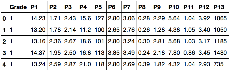
The proposed dataset can be downloaded here . Reference to the source data and description of the signs will be at the end of the article. According to the presented parameters, we are invited to determine what kind of wine this or that wine belongs to. Now we can figure out what is happening there:
Working in Jupyter notebook, we get this answer:
This means that now we have data available for analysis. In the first column, the Grade values show which wine belongs to, and the remaining columns are indications by which they can be distinguished. Try typing data instead of data.head () - now you can see not only the “upper part” of the dataset.
We turn to the main part of the article - we solve the problem of classification. All in order:
Let's look at the implementation (each excerpt from the code is a separate Cell in the notebook):
We create arrays, where X - signs (1 to 13 columns), y - classes (0th column). Then, to build a test and training sample from the source data, we use the convenient cross-validation function train_test_split , implemented in scikit-learn. We work further with ready samples - import the RandomForestClassifier from ensemble into sklearn. This class contains all the methods and functions necessary for learning and testing the machine. We assign the RandomForestClassifier class to the clf (classifier) variable, then we train the machine from the clf class by calling the fit () function, where X_train are signs of the y_train categories. You can now use the built-in score metric in the class to determine the accuracy of the categories predicted for X_test from the true values of these categories y_test . When using this metric, the accuracy value is displayed from 0 to 1, where 1 <=> 100% Done!
- Quite good accuracy. Does that always happen?
For solving classification problems, an important factor is the selection of the best parameters for a training sample of categories. The bigger, the better. But not always (you can also read about this in more detail on the Internet, however, most likely, I will write about this one more article designed for beginners).
- Too easy. More meat!
For a visual viewing of the learning result on this dataset, you can give an example: leaving only two parameters to set them in two-dimensional space, we construct a graph of the trained sample (we get something like this, it depends on the learning):
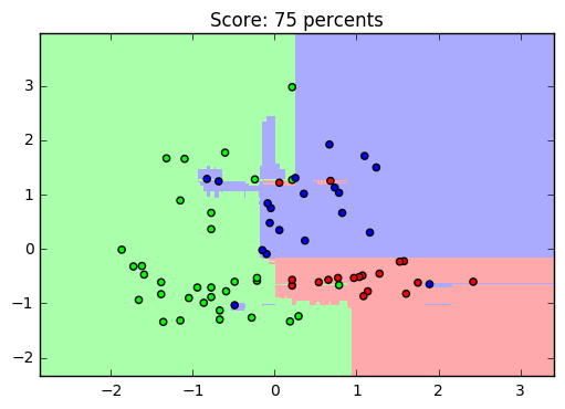
Yes, with a decrease in the number of signs, the accuracy of recognition also decreases. And the graph turned out to be not particularly beautiful, but it is not decisive in a simple analysis: it is quite clearly seen how the machine selected the training sample (points) and compared it with the predicted (fill) values.
I suggest the reader to find out for himself why and how he works.
I hope this article has helped you get a little comfortable in developing simple machine learning in Python. This knowledge will be enough to continue an intensive course on further studying BigData + Machine Learning. The main thing is to move from simple to in-depth gradually. But useful resources and articles, as promised:
Historical essays:
More about machine learning:
We study python, or to work with data:
However, knowledge of English will be useful for the best mastering of the sklearn library: this source contains all the necessary knowledge (since this is API reference).
A more in-depth study of the use of machine learning with Python has become possible, and simpler thanks to teachers from Yandex - this course has all the necessary means of explaining how the whole system works, describes more about the types of machine learning, and so on.
The file of today's dataset was taken from here and somewhat modified.
Where to get data, or "dataset storage" - here a huge amount of data from a variety of sources is collected. It is very useful to train on real data.
I would be grateful for the support to improve this article, as well as I am ready for any kind of constructive criticism.
Who is this article for?
Anyone who would be interested then to delve into the history of searching for new facts, or anyone who wondered at least once the question “how does all this, machine learning, work,” will find here the answer to his question. Most likely, an experienced reader will not find anything interesting for himself here, since the software part
In numbers
Every year there is a growing need for exploring big data, both for companies and for active enthusiasts. In large companies such as Yandex or Google, data tools such as the R programming language or libraries for Python are increasingly used (in this article I cite examples written under Python 3). According to Moore's Law (and in the picture, he himself), the number of transistors on an integrated circuit doubles every 24 months. This means that every year the productivity of our computers grows, which means that the previously inaccessible boundaries of knowledge are again “shifted to the right” - there is open space for studying big data, which is primarily connected with the creation of a “science of big data”, which Mostly it became possible due to the application of the previously described machine learning algorithms, which could only be verified after half a century. Who knows, maybe in a few years we will be able to describe in absolute accuracy various forms of fluid movement, for example.
Is data analysis easy?
Yes. And just as interesting. Along with the special importance for all of humanity to study big data, there is a relative simplicity in studying them independently and applying the received “answer” (from an enthusiast to enthusiasts). To solve the problem of classification today there is a huge amount of resources; omitting most of them, you can use the tools library Scikit-learn (SKlearn). Create your first training machine:
')
clf = RandomForestClassifier() clf.fit(X, y) So we created a simple machine that can predict (or classify) the values of arguments by their attributes.
- If everything is so simple, why still not everyone predicts, for example, currency prices?
With these words, it would be possible to finish the article, but
Closer to the point
- It turns out, I cannot earn this business right away?
Yes, we are still far away from solving problems for prizes of $ 100,000, but everyone started with something simple.
So today we will need:
- Python 3 (with pip3 installed)
- Jupyter
- SKlearn, NumPy and matplotlib
If something is not: we put everything in 5 minutes
First of all, download and install Python 3 (during installation, do not forget to install pip and add it to PATH if you downloaded the Windows installer). Then, for convenience, the Anaconda package was taken and used, which includes more than 150 libraries for Python (download link ). It is convenient for use by Jupyter, the numpy, scikit-learn, matplotlib libraries, and also simplifies the installation of all. After installation, launch Jupyter Notebook via the Anaconda control panel, or via the command line (terminal): “jupyter notebook”.
Further use requires some knowledge of the Python syntax and its capabilities from the reader (at the end of the article there will be links to useful resources, among them “the basics of Python 3”).
As usual, we import the necessary libraries for work:
import numpy as np from pandas import read_csv as read - Ok, with Numpy everything is clear. But why do we need Pandas, and also read_csv?
Sometimes it is convenient to “visualize” existing data, then it becomes easier to work with them. Moreover, most datasets from the popular Kaggle service are collected by users in CSV format.
This is how it is rendered by pandas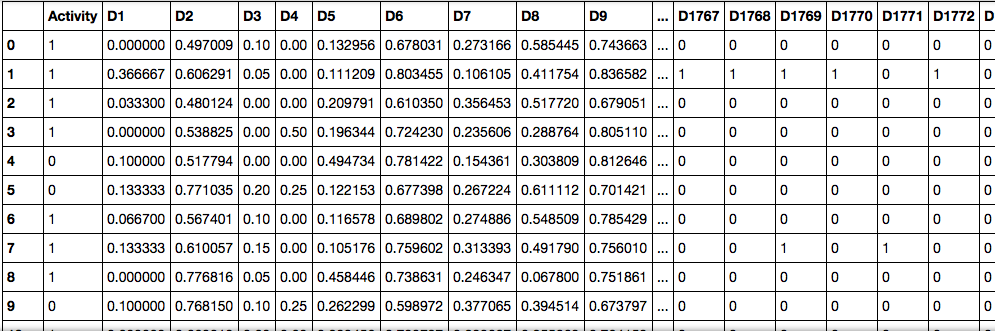
Here the Activity column shows whether the reaction is going on or not (1 for a positive, 0 for a negative). And the remaining columns - sets of signs and the corresponding values (different percentages of substances in the reaction, their state of aggregation, etc.)
Here the Activity column shows whether the reaction is going on or not (1 for a positive, 0 for a negative). And the remaining columns - sets of signs and the corresponding values (different percentages of substances in the reaction, their state of aggregation, etc.)
- I remember you used the word "dataset". So what is it?
Dataset is a sample of data, usually in the format of “a set of signs” → “some values” (which may be, for example, housing prices, or the sequence number of a set of some classes), where X is a set of signs, and y are some values. For example, determining the correct indices for a set of classes is the task of classification , and finding target values (such as price, or distances to objects) is the task of ranking . More information about the types of machine learning can be found in articles and publications, links to which, as promised, will be at the end of the article.
We get acquainted with the data
The proposed dataset can be downloaded here . Reference to the source data and description of the signs will be at the end of the article. According to the presented parameters, we are invited to determine what kind of wine this or that wine belongs to. Now we can figure out what is happening there:
path = "% %/wine.csv" data = read(path, delimiter=",") data.head() Working in Jupyter notebook, we get this answer:
This means that now we have data available for analysis. In the first column, the Grade values show which wine belongs to, and the remaining columns are indications by which they can be distinguished. Try typing data instead of data.head () - now you can see not only the “upper part” of the dataset.
Simple implementation of the classification task
We turn to the main part of the article - we solve the problem of classification. All in order:
- create a training set
- we try to train the car on randomly selected parameters and classes corresponding to them
- calculate the quality of the sold machine
Let's look at the implementation (each excerpt from the code is a separate Cell in the notebook):
X = data.values[::, 1:14] y = data.values[::, 0:1] from sklearn.cross_validation import train_test_split as train X_train, X_test, y_train, y_test = train(X, y, test_size=0.6) from sklearn.ensemble import RandomForestClassifier clf = RandomForestClassifier(n_estimators=100, n_jobs=-1) clf.fit(X_train, y_train) clf.score(X_test, y_test) We create arrays, where X - signs (1 to 13 columns), y - classes (0th column). Then, to build a test and training sample from the source data, we use the convenient cross-validation function train_test_split , implemented in scikit-learn. We work further with ready samples - import the RandomForestClassifier from ensemble into sklearn. This class contains all the methods and functions necessary for learning and testing the machine. We assign the RandomForestClassifier class to the clf (classifier) variable, then we train the machine from the clf class by calling the fit () function, where X_train are signs of the y_train categories. You can now use the built-in score metric in the class to determine the accuracy of the categories predicted for X_test from the true values of these categories y_test . When using this metric, the accuracy value is displayed from 0 to 1, where 1 <=> 100% Done!
About RandomForestClassifier and cross-validation method train_test_split
During clf initialization for RandomForestClassifier, we set the values n_estimators = 100, n_jobs = -1 , where the first is responsible for the number of trees in the forest and the second for the number of processor cores involved (with all cores involved, the default is 1). Since we are working with this dataset and we have nowhere to take a test sample, we use train_test_split to “ cleverly ” split the data into a training sample and test. You can learn more about them by highlighting the class or method you are interested in and pressing Shift + Tab in the Jupyter environment.
- Quite good accuracy. Does that always happen?
For solving classification problems, an important factor is the selection of the best parameters for a training sample of categories. The bigger, the better. But not always (you can also read about this in more detail on the Internet, however, most likely, I will write about this one more article designed for beginners).
- Too easy. More meat!
For a visual viewing of the learning result on this dataset, you can give an example: leaving only two parameters to set them in two-dimensional space, we construct a graph of the trained sample (we get something like this, it depends on the learning):
Yes, with a decrease in the number of signs, the accuracy of recognition also decreases. And the graph turned out to be not particularly beautiful, but it is not decisive in a simple analysis: it is quite clearly seen how the machine selected the training sample (points) and compared it with the predicted (fill) values.
Implementation here
from sklearn.preprocessing import scale X_train_draw = scale(X_train[::, 0:2]) X_test_draw = scale(X_test[::, 0:2]) clf = RandomForestClassifier(n_estimators=100, n_jobs=-1) clf.fit(X_train_draw, y_train) x_min, x_max = X_train_draw[:, 0].min() - 1, X_train_draw[:, 0].max() + 1 y_min, y_max = X_train_draw[:, 1].min() - 1, X_train_draw[:, 1].max() + 1 h = 0.02 xx, yy = np.meshgrid(np.arange(x_min, x_max, h), np.arange(y_min, y_max, h)) pred = clf.predict(np.c_[xx.ravel(), yy.ravel()]) pred = pred.reshape(xx.shape) import matplotlib.pyplot as plt from matplotlib.colors import ListedColormap cmap_light = ListedColormap(['#FFAAAA', '#AAFFAA', '#AAAAFF']) cmap_bold = ListedColormap(['#FF0000', '#00FF00', '#0000FF']) plt.figure() plt.pcolormesh(xx, yy, pred, cmap=cmap_light) plt.scatter(X_train_draw[:, 0], X_train_draw[:, 1], c=y_train, cmap=cmap_bold) plt.xlim(xx.min(), xx.max()) plt.ylim(yy.min(), yy.max()) plt.title("Score: %.0f percents" % (clf.score(X_test_draw, y_test) * 100)) plt.show() I suggest the reader to find out for himself why and how he works.
The last word
I hope this article has helped you get a little comfortable in developing simple machine learning in Python. This knowledge will be enough to continue an intensive course on further studying BigData + Machine Learning. The main thing is to move from simple to in-depth gradually. But useful resources and articles, as promised:
Materials that inspired the author to create this article
Historical essays:
- An article about why machine learning is needed today, and what led to this
- Oddly enough, rather intricate article from Wikipedia about machine learning in general
More about machine learning:
We study python, or to work with data:
- Very useful course from talented teachers from ITMO and SPbAU
- An excellent Russian-language resource for learners of Python, but poorly oriented to English-speaking resources.
However, knowledge of English will be useful for the best mastering of the sklearn library: this source contains all the necessary knowledge (since this is API reference).
A more in-depth study of the use of machine learning with Python has become possible, and simpler thanks to teachers from Yandex - this course has all the necessary means of explaining how the whole system works, describes more about the types of machine learning, and so on.
The file of today's dataset was taken from here and somewhat modified.
Where to get data, or "dataset storage" - here a huge amount of data from a variety of sources is collected. It is very useful to train on real data.
I would be grateful for the support to improve this article, as well as I am ready for any kind of constructive criticism.
Source: https://habr.com/ru/post/319288/
All Articles