Simple FDTD implementation in Java
FDTD ( Finite Difference Time Domain ) - the method of finite differences in the time domain - the most "honest" method for solving the problem of electrodynamics from low frequencies to the visible range. The essence is the solution of Maxwell's equations "head on." It is well painted. Especially look at the grid.
The problem was solved in the two-dimensional case by a simple explicit difference scheme. I don't like implicit schemes, and they require a lot of memory. Calculation with normal accuracy requires small pitch grids, as compared with simpler methods, a lot of time is required. Therefore, maximum emphasis was placed on performance.
Presents the implementation of the algorithm in Java and C ++.
')

About six years, my main language for calculations and trifles was Matlab. The reason is the simplicity of writing and visualizing the result. And since I switched from Borland C ++ 3.1, the progress of the possibilities was obvious. (In Python, I never fumbled, but in C ++ then weakly).
I needed FDTD for calculations as a reliable and reliable method. Began to study the issue in 2010-11. Available packages or it was not clear how to use, or did not know what I needed. I decided to write my own program for precise control over everything. After reading the classic article “ Numerical solution of Maxwell’s equations in isotropic media ”, he wrote a three-dimensional case, but then simplified it to a two-dimensional one. Why 3D is difficult, I will explain later.
Then he optimized and simplified the Matlab code as much as possible. After all the improvements, it turned out that the 2000x2000 grid runs in 107 minutes. At i5-3.8 GHz. Then this speed was enough. The useful thing was that the calculation of complex fields immediately took place in Matlab, and it was easy to show pictures of the spread. Also, everything was considered to be in doubles, because the Matlab's speed practically had no effect. Yes, my standard calculation is one pass of light through a photonic crystal.
There were two problems. It was necessary to calculate the spectra with high accuracy, and to do this, use a large grid width. A physical increase in the area in both coordinates by 2 times increases the calculation time by 8 times (crystal size * time of passage).
I continued to use Matlab, but became a Java programmer. And, comparing the performance of different algorithms, he began to suspect something . For example, bubble sorting - only loops, arrays and comparisons - in Matlab is 6 times slower than in C ++ or Java. And this is still good for him. The five-dimensional cycle for the Euler conjecture in Matlab is 400 times longer.
First I started writing FDTD in C ++. There was an embedded std :: complex. But then I abandoned this idea. (In Matlab, not such brackets, copy-paste did not work, I had to spend a drop of time). Now I checked C ++ - complex mathematics gives speed loss 5 times . It's too much. As a result, wrote in Java.
A little about the question "Why Java?". I will describe the performance details later. In short, in simple non-OOP code, only arithmetic and cycles are C ++ with O3 optimization or the same speed, or up to + 30% faster. I just know better now how to understand Java, interface and work with graphics.
We now turn to the code. I will try to show everything, with explanations of the problem and the algorithm. In the two-dimensional case, the Maxwell system of equations splits into two independent subsystems - TE and TM waves. The code is shown for TE. There are 3 components - electric field Ez and magnetic Hx, Hy. To simplify the time has the dimension of meters.
Initially, I thought that there was no point in float, since all calculations are reduced to double. Therefore, I will give the code for double - it is less than the excess. All arrays have dimensions of +1, so that the indices coincide with the Matlab matrices (from 1, not from 0).
Somewhere in the start code:
The main method:
Initialization of the dielectric constant (crystal lattice). More precisely, the return value with constants. A discrete function is used (0 or 1). It seems to me closer to real samples. Of course, you can write anything here:
The crystal lattice looks like this:

Arrays used for boundary conditions:
Count limit on time. Since we have a step dt = dx / 2, the standard coefficient is 2. If the medium is dense, or you need to go at an angle - more.
We start the main loop:
The variable tt here takes into account the speed limit of light, with a small margin. We will consider only the area where the light could reach.
Instead of complex numbers, I consider two components separately - sine and cosine. I thought that for speed it's better to copy a piece than to make a choice inside the loop. Perhaps replace the function call or lambda.
Here, at our entrance to the region (to the leftmost coordinate), a Gaussian beam of half-width w enters, at an angle α, oscillating in time. This is exactly how the “laser” radiation of the required frequency / wavelength appears.
Then we copy the temporary arrays under Moore’s absorbing boundary conditions :
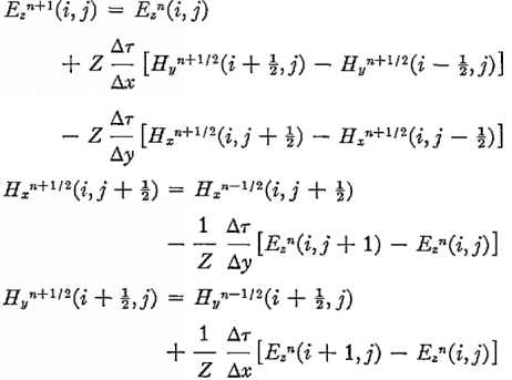
Now we go to the main calculation - the next step across the field. The peculiarity of Maxwell's equations is that the time variation of the magnetic field depends only on the electric one and vice versa. This allows you to write a simple difference scheme. The initial formulas were as follows:
I recalculated all the extra constants in advance, replaced the dimension H, introduced and took into account the dielectric constant. Since the original formulas for the grid shifted by 0.5, you need not make a mistake with the indices of the arrays E and N. They are of different lengths - E is 1 more.
Cycle area for E:
And now finally apply the boundary conditions. They are needed because the difference scheme does not consider extreme cells - there are no formulas for them. If you do nothing, the light will be reflected from the walls. Therefore, we use the method that minimizes reflection in a normal fall. We process three sides - top, bottom and right. The loss of productivity on the boundary conditions is about 1% (the smaller, the larger the task).
On the left is a special border - a ray is generated in it. Just like last time. Just 1 step further in time.
It remains only to calculate the magnetic field:
And little things: pass the final segment to calculate the Fourier transform - finding the picture in the far zone (direction space):
Separately, we take the Fourier transform:
Since I do not understand fast Fourier, I took the first one I got . Minus - width is only a power of two.
We turn to the most interesting for me - what good we have received by moving from Matlab to Java. In Matlab I once optimized everything I could. In Java, it is mostly an internal loop (complexity n ^ 3). Matlab has already taken into account that he considers two components at once. Speed in the first stage (more is better):
UPD. Added the result of Matlab, in which he replaced the double cycles with the subtraction of matrices.
We describe the main participants of the competition.
At first, I considered the TE and TM components sequentially. By the way, this is the only option with a lack of memory. Then he wrote two threads - simple Runnable. Here are just a little progress. Only 20-22% faster than 1-flow. Started looking for reasons. Threads worked fine. 2 cores were stably loaded at 100%, not allowing the laptop to live.
Then I counted the performance. It turned out that it rests on the speed of RAM. The code was already working at the limit of reading. "I had to" switch to float . An accuracy check showed that there were no deadly errors. There is definitely no visual difference. The total energy differed in the 8th sign. After the integral transformation, the maximum of the spectrum is at 0.7e-6. Perhaps, the fact is that Java considers everything in 64-bit precision, and only then it converts to 32.
But the main thing - got a performance spurt. The total effect of 2 cores and the transition to float + 87–102%. (The faster the memory and the more cores, the better the gain). Athlon x3 gave little gain.
The implementation in C ++ is similar - through std :: thread (see the end).
Current speeds (2 threads):
(new compilers provide very high performance, compared to Java, on 16384. Java and GCC-4.9 32 fail in this case).
All evaluations were performed for a single run calculation. Because, if you re-run from the GUI, without closing the program, the speed further increases. IMHO, jit-optimization taxis.
It seemed to me that there was still much to accelerate. I started on the 4-way version. Essence - the region is divided in half and counted in 2 streams, first along E, then along N.
I first wrote it on Runnable. It turned out terribly - acceleration was only for a very large width of the area. Excessive costs of spawning new streams. Then I mastered java.util.concurrent. Now I had a fixed pool of threads that were given tasks:
Inside the thread, the loop is executed.
A similar class for H is just different boundaries and its own cycle.
Now there is always a gain from 4 streams - from 23 to 49% (.jar). The smaller the width, the better - judging by the speed, we get into the cache memory. The greatest benefit will be if we consider the long narrow tasks.
The C ++ implementation so far contains only simple std :: thread. Therefore, for her, the wider, the better. Acceleration of C ++ from 5% with a width of 1024 to 47% at 16384.
UPD. Added results of GCC 6.2-64 and VisualStudio. VS is faster than old GCC by 13–43%, new by 3–11%. The main features of 64-bit compilers are faster work on wide tasks. Also, since Java is better parallelized on small tasks (cache), and C ++ on broad tasks - on broad tasks Visual Studio is 61% faster than Java.
As we can see, in the best case, Java growth by 49% is like almost 3 cores. Therefore, we have a funny fact - for small tasks it is best to set newFixedThreadPool (3);
For large - by the number of threads in the processor - 4 or 6-8. I will point out another funny fact. On Athlone x3 there was very little progress from the transition to float and 2 streams - 32% of both optimizations. The gain from the "4" -nuclear code in C ++ is also small - 67% between 1 and 4 cores (both float). You can write off on a slow memory controller and 32-bit Windu.
But the 4-core Java code worked fine. With 3 Executor threads + 50.2% of the 2-core version for large tasks. For some reason, the worst 2-core implementation has intensified as much as possible multi-core.
Last note on 4-core code in Java. Current time spent:
I tried to optimize the main cycles as much as possible, thinking that the rest is spending little time.
I also post the full code of the 4-core case in C ++:
This is the simplest code, without a normal lattice and boundary conditions. It is interesting, is it possible in C ++ to more effectively declare 2-dimensional arrays and call threads?
And I have no more cores. If my tasks did not rest on the memory, I would divide further. It seems, ThreadPool gives small expenses. Or go to the Fork-Join Framework.
I could check - abandon the first two streams, and divide one task into 4-8 pieces on i7. But it only makes sense if someone tests on a machine with fast memory - DDR-4 or 4 channels.
The best way to get rid of the lack of memory speed is with a video card. My brother, who forbids updating the video driver (ignorance of C and Cuda), prevents me from switching to Cuda.
I can quickly solve any 2-dimensional task I need with good accuracy. The grid 4096x2000 is passed on a 4-core in 106 seconds. It will be 300 microns x 40 layers - we have the maximum samples.
In 2D, with 32-bit precision, some memory is required - 4 bytes * 4 arrays * 2 complex components = 32 bytes / pixel in the worst case.
In 3D, everything is much worse. Component already six. You can opt out of two threads - read the components sequentially and write on the screw. You can not store an array of dielectric constant, and count in a cycle or get along with a very small periodic area. Then in 16 GB of operatives (the maximum is on my work) the area 895x895x895 will fit. It will be fine "to see." But it will be considered “only” 6–7 hours one pass. If the task is well divided into 4 parallel threads. And if we neglect the calculation of ε.
Only for the spectrum is not enough for me. With a width of 1024, I do not see the necessary details. You need 2048. And this is 200+ GB of memory. Therefore, the three-dimensional case is difficult. If you do not develop a code with caching SSD.
PS Speed estimates were rather approximate. I checked Matlab only on small problems. Now I checked Java - task 2048 * 1976 (analog 2000 * 2000) on 4 cores. Calculation time is 45.5 seconds. Acceleration from Matlab 141 times (exactly).
*) Check the speed of pure C (not ++). By benchmarksgame he is always faster.
1) Check out complex classes in C and Java. Maybe in C they are implemented fairly quickly. True, I'm afraid they will all be more than 8 bytes.
2) Throw all 2- and 4-core versions in MSVS, find the optimization settings.
3) Check if lyabmdy / stream can speed up the main loop or additional.
4) Make a normal GUI for selecting everything and visualizing the results.
99) Write a Cuda version.
If anyone is interested, I will describe FDTD and other calculation methods, photonic crystals.
I posted 2 versions on Github:
1) 2-way with the rudiments of the parameter selection interface
2) 4-way
Both draw a picture and spectrum. Just until a pixel is in a pixel - do not take the width above 2048. They also know how to take the size of the area from the console.
The problem was solved in the two-dimensional case by a simple explicit difference scheme. I don't like implicit schemes, and they require a lot of memory. Calculation with normal accuracy requires small pitch grids, as compared with simpler methods, a lot of time is required. Therefore, maximum emphasis was placed on performance.
Presents the implementation of the algorithm in Java and C ++.
')
Foreword
About six years, my main language for calculations and trifles was Matlab. The reason is the simplicity of writing and visualizing the result. And since I switched from Borland C ++ 3.1, the progress of the possibilities was obvious. (In Python, I never fumbled, but in C ++ then weakly).
I needed FDTD for calculations as a reliable and reliable method. Began to study the issue in 2010-11. Available packages or it was not clear how to use, or did not know what I needed. I decided to write my own program for precise control over everything. After reading the classic article “ Numerical solution of Maxwell’s equations in isotropic media ”, he wrote a three-dimensional case, but then simplified it to a two-dimensional one. Why 3D is difficult, I will explain later.
Then he optimized and simplified the Matlab code as much as possible. After all the improvements, it turned out that the 2000x2000 grid runs in 107 minutes. At i5-3.8 GHz. Then this speed was enough. The useful thing was that the calculation of complex fields immediately took place in Matlab, and it was easy to show pictures of the spread. Also, everything was considered to be in doubles, because the Matlab's speed practically had no effect. Yes, my standard calculation is one pass of light through a photonic crystal.
There were two problems. It was necessary to calculate the spectra with high accuracy, and to do this, use a large grid width. A physical increase in the area in both coordinates by 2 times increases the calculation time by 8 times (crystal size * time of passage).
I continued to use Matlab, but became a Java programmer. And, comparing the performance of different algorithms, he began to suspect something . For example, bubble sorting - only loops, arrays and comparisons - in Matlab is 6 times slower than in C ++ or Java. And this is still good for him. The five-dimensional cycle for the Euler conjecture in Matlab is 400 times longer.
First I started writing FDTD in C ++. There was an embedded std :: complex. But then I abandoned this idea. (In Matlab, not such brackets, copy-paste did not work, I had to spend a drop of time). Now I checked C ++ - complex mathematics gives speed loss 5 times . It's too much. As a result, wrote in Java.
A little about the question "Why Java?". I will describe the performance details later. In short, in simple non-OOP code, only arithmetic and cycles are C ++ with O3 optimization or the same speed, or up to + 30% faster. I just know better now how to understand Java, interface and work with graphics.
FDTD - more details
We now turn to the code. I will try to show everything, with explanations of the problem and the algorithm. In the two-dimensional case, the Maxwell system of equations splits into two independent subsystems - TE and TM waves. The code is shown for TE. There are 3 components - electric field Ez and magnetic Hx, Hy. To simplify the time has the dimension of meters.
Initially, I thought that there was no point in float, since all calculations are reduced to double. Therefore, I will give the code for double - it is less than the excess. All arrays have dimensions of +1, so that the indices coincide with the Matlab matrices (from 1, not from 0).
Somewhere in the start code:
public static int nx = 4096;// . 2 . public static int ny = 500;// The main method:
Initialization of initial variables
public static double[][] callFDTD(int nx, int ny, String method) { int i, j;// double x; // final double lambd = 1064e-9; // final double dx = lambd / 15; // . λ/10. , . final double dy = dx; // . final double period = 2e-6; // final double Q = 1.0;// final double n = 1;// final double prodol = 2 * n * period * period / lambd / Q; // final double omega = 2 * PI / lambd; // final double dt = dx / 2; // . , final double tau = 2e-5 * 999;// . . , . final double s = dt / dx; // final double k3 = (1 - s) / (1 + s);// final double w = 19e-7;// final double alpha = sin(0.0 / 180 * PI);// . . double[][] Ez = new double[nx + 1][ny + 1]; double[][] Hx = new double[nx][ny]; // double[][] Hy = new double[nx][ny]; final int begin = 10; // , . . final double mod = 0.008 * 2;// = 2*Δn; final double ds = dt * dt / dx / dx;// Initialization of the dielectric constant (crystal lattice). More precisely, the return value with constants. A discrete function is used (0 or 1). It seems to me closer to real samples. Of course, you can write anything here:
double[][] e = new double[nx + 1][ny + 1]; for (i = 1; i < nx + 1; i++) { for (j = 1; j < ny + 1; j++) { e[i][j] = ds / (n + ((j < begin) ? 0 : (mod / 2) * (1 + signum(-0.1 + cos(2 * PI * (i - nx / 2.0 + 0.5) * dx / period) * sin(2 * PI * (j - begin) * dy / prodol))))); } } The crystal lattice looks like this:
Arrays used for boundary conditions:
double[][] end = new double[2][nx + 1]; double[][] top = new double[2][ny + 1]; double[][] bottom = new double[2][ny + 1]; Count limit on time. Since we have a step dt = dx / 2, the standard coefficient is 2. If the medium is dense, or you need to go at an angle - more.
final int tMax = (int) (ny * 2.2); We start the main loop:
for (int t = 1; t <= tMax; t++) { double tt = Math.min(t * s + 10, ny - 1); The variable tt here takes into account the speed limit of light, with a small margin. We will consider only the area where the light could reach.
Instead of complex numbers, I consider two components separately - sine and cosine. I thought that for speed it's better to copy a piece than to make a choice inside the loop. Perhaps replace the function call or lambda.
switch (method) { case "cos": for (i = 1; i <= nx - 1; i++) { x = dx * (i - (double) nx / 2 + 0.5); // Ez[i][1] = exp(-pow(x, 2) / w / w - (t - 1) * dt / tau) * cos((x * alpha + (t - 1) * dt) * omega); } break; sin
case "sin": for (i = 1; i <= nx - 1; i++) { x = dx * (i - (double) nx / 2 + 0.5); Ez[i][1] = exp(-pow(x, 2) / w / w - (t - 1) * dt / tau) * sin((x * alpha + (t - 1) * dt) * omega); } break; } Here, at our entrance to the region (to the leftmost coordinate), a Gaussian beam of half-width w enters, at an angle α, oscillating in time. This is exactly how the “laser” radiation of the required frequency / wavelength appears.
Then we copy the temporary arrays under Moore’s absorbing boundary conditions :
for (i = 1; i <= nx; i++) { end[0][i] = Ez[i][ny - 1]; end[1][i] = Ez[i][ny]; } System.arraycopy(Ez[1], 0, top[0], 0, ny + 1); System.arraycopy(Ez[2], 0, top[1], 0, ny + 1); System.arraycopy(Ez[nx - 1], 0, bottom[0], 0, ny + 1); System.arraycopy(Ez[nx], 0, bottom[1], 0, ny + 1); Now we go to the main calculation - the next step across the field. The peculiarity of Maxwell's equations is that the time variation of the magnetic field depends only on the electric one and vice versa. This allows you to write a simple difference scheme. The initial formulas were as follows:
I recalculated all the extra constants in advance, replaced the dimension H, introduced and took into account the dielectric constant. Since the original formulas for the grid shifted by 0.5, you need not make a mistake with the indices of the arrays E and N. They are of different lengths - E is 1 more.
Cycle area for E:
for (i = 2; i <= nx - 1; i++) { for (j = 2; j <= tt; j++) {// ? Ez[i][j] += e[i][j] * ((Hx[i][j - 1] - Hx[i][j] + Hy[i][j] - Hy[i - 1][j])); } } And now finally apply the boundary conditions. They are needed because the difference scheme does not consider extreme cells - there are no formulas for them. If you do nothing, the light will be reflected from the walls. Therefore, we use the method that minimizes reflection in a normal fall. We process three sides - top, bottom and right. The loss of productivity on the boundary conditions is about 1% (the smaller, the larger the task).
for (i = 1; i <= nx; i++) { Ez[i][ny] = end[0][i] + k3 * (end[1][i] - Ez[i][ny - 1]);//end } for (i = 1; i <= ny; i++) { Ez[1][i] = top[1][i] + k3 * (top[0][i] - Ez[2][i]);//verh kray Ez[nx][i] = bottom[0][i] + k3 * (bottom[1][i] - Ez[nx - 1][i]); } On the left is a special border - a ray is generated in it. Just like last time. Just 1 step further in time.
Laser
switch (method) { case "cos": for (i = 1; i <= nx - 1; i++) { x = dx * (i - (double) nx / 2 + 0.5); Ez[i][1] = exp(-pow(x, 2) / w / w - (t - 1) * dt / tau) * cos((x * alpha + t * dt) * omega); } break; case "sin": for (i = 1; i <= nx - 1; i++) { x = dx * (i - (double) nx / 2 + 0.5); Ez[i][1] = exp(-pow(x, 2) / w / w - (t - 1) * dt / tau) * sin((x * alpha + t * dt) * omega); } break; } It remains only to calculate the magnetic field:
for (i = 1; i <= nx - 1; i++) { // main Hx Hy for (j = 1; j <= tt; j++) { Hx[i][j] += Ez[i][j] - Ez[i][j + 1]; Hy[i][j] += Ez[i + 1][j] - Ez[i][j]; } } } // 3- . And little things: pass the final segment to calculate the Fourier transform - finding the picture in the far zone (direction space):
int pos = method.equals("cos") ? 0 : 1; // BasicEx.forFurier[pos] = new double[nx]; // int endF = (int) (ny * 0.95);// for (i = 1; i <= nx; i++) { BasicEx.forFurier[pos][i - 1] = Ez[i][endF]; for (j = 1; j <= ny; j++) { Ez[i][j] = abs(Ez[i][j]);// ABS } // , - } Hx = null; // , Hy = null; e = null; return Ez; } Then we put the squares of the two components, and display the intensity image.
for (int i = 0; i < nx + 1; i++) { for (int j = 0; j < ny + 1; j++) { co.E[i][j] = co.E[i][j] * co.E[i][j] + si.E[i][j] * si.E[i][j]; } } Separately, we take the Fourier transform:
fft.fft(forFurier[0], forFurier[1]); Since I do not understand fast Fourier, I took the first one I got . Minus - width is only a power of two.
About performance
We turn to the most interesting for me - what good we have received by moving from Matlab to Java. In Matlab I once optimized everything I could. In Java, it is mostly an internal loop (complexity n ^ 3). Matlab has already taken into account that he considers two components at once. Speed in the first stage (more is better):
| Matlab | one |
| Matlab matrix | 3.4 / 5.1 (float) |
| Java double | 50 |
| C ++ gcc double | 48 |
| C ++ MSVS double | 55 |
| C ++ gcc float | 73 |
| C ++ MSVS float | 79 |
UPD. Added the result of Matlab, in which he replaced the double cycles with the subtraction of matrices.
We describe the main participants of the competition.
- Matlab - 2011b and 2014. The transition to 32-bit numbers gives a very small increase in speed.
- Java is at first 7u79, but mostly 8u102. It seemed to me that 8 was slightly better, but did not compare in detail.
- Microsoft VisualStudio 2015 release configuration
- MinGW, gcc 4.9.2 32 bit, December 2014, always O3 optimization. march = core i7, without AVX. AVX on my laptop is not there, where there is a growth did not give.
Test machines:
- Pentium 2020m 2.4 GHz, ddr3-1600 1 channel
- Core i5-4670 3.6–3.8 GHz, ddr3-1600 2 channels
- Core i7-4771 3.7–3.9 GHz, ddr3-1333 2 channels
- Athlon x3 3.1 GHz, ddr3-1333, very slow memory controller.
2-core stage
At first, I considered the TE and TM components sequentially. By the way, this is the only option with a lack of memory. Then he wrote two threads - simple Runnable. Here are just a little progress. Only 20-22% faster than 1-flow. Started looking for reasons. Threads worked fine. 2 cores were stably loaded at 100%, not allowing the laptop to live.
Then I counted the performance. It turned out that it rests on the speed of RAM. The code was already working at the limit of reading. "I had to" switch to float . An accuracy check showed that there were no deadly errors. There is definitely no visual difference. The total energy differed in the 8th sign. After the integral transformation, the maximum of the spectrum is at 0.7e-6. Perhaps, the fact is that Java considers everything in 64-bit precision, and only then it converts to 32.
But the main thing - got a performance spurt. The total effect of 2 cores and the transition to float + 87–102%. (The faster the memory and the more cores, the better the gain). Athlon x3 gave little gain.
The implementation in C ++ is similar - through std :: thread (see the end).
Current speeds (2 threads):
| Java double | 61 |
| Java float | 64-101 |
| C ++ gcc float | 87-110 |
| C ++ gcc 6.2 64 native | 99-122 |
| Visual studio | 112- 149 |
(new compilers provide very high performance, compared to Java, on 16384. Java and GCC-4.9 32 fail in this case).
All evaluations were performed for a single run calculation. Because, if you re-run from the GUI, without closing the program, the speed further increases. IMHO, jit-optimization taxis.
4-core stage
It seemed to me that there was still much to accelerate. I started on the 4-way version. Essence - the region is divided in half and counted in 2 streams, first along E, then along N.
I first wrote it on Runnable. It turned out terribly - acceleration was only for a very large width of the area. Excessive costs of spawning new streams. Then I mastered java.util.concurrent. Now I had a fixed pool of threads that were given tasks:
public static ExecutorService service = Executors.newFixedThreadPool(4); //…… cdl = new CountDownLatch(2); NewThreadE first = new NewThreadE(Ez, Hx, Hy, e, 2, nx / 2, tt, cdl); NewThreadE second = new NewThreadE(Ez, Hx, Hy, e, nx / 2 + 1, nx - 1, tt, cdl); service.execute(first); service.execute(second); try { cdl.await(); } catch (InterruptedException ex) { } And for H:
cdl = new CountDownLatch(2); NewThreadH firstH = new NewThreadH(Ez, Hx, Hy, 1, nx / 2, tt, cdl); NewThreadH secondH = new NewThreadH(Ez, Hx, Hy, nx/2+1, nx-1, tt, cdl); service.execute(firstH); service.execute(secondH); try { cdl.await(); } catch (InterruptedException ex) { } Inside the thread, the loop is executed.
class NewThreadE
public class NewThreadE implements Runnable { float[][] Ez; float[][] Hx; float[][] Hy; float[][] e; int iBegin; int iEnd; float tt; CountDownLatch cdl; public NewThreadE(float[][] E, float[][] H, float[][] H2, float[][] eps, int iBegi, int iEn, float ttt, CountDownLatch cdl) { this.cdl = cdl; Ez = E; Hx = H; Hy = H2; e = eps; iBegin = iBegi; iEnd = iEn; tt = ttt; } @Override public void run() { for (int i = iBegin; i <= iEnd; i++) { // main Ez for (int j = 2; j <= tt; j++) { Ez[i][j] += e[i][j] * ((Hx[i][j - 1] - Hx[i][j] + Hy[i][j] - Hy[i - 1][j])); } } cdl.countDown(); } } A similar class for H is just different boundaries and its own cycle.
Now there is always a gain from 4 streams - from 23 to 49% (.jar). The smaller the width, the better - judging by the speed, we get into the cache memory. The greatest benefit will be if we consider the long narrow tasks.
| Java float 4 threads | 86–151 |
| C ++ gcc float 4flow | 122–162 (closer to 128) |
| C ++ gcc 6.2 64 native | 124–173 |
| Visual studio | 139–183 |
The C ++ implementation so far contains only simple std :: thread. Therefore, for her, the wider, the better. Acceleration of C ++ from 5% with a width of 1024 to 47% at 16384.
UPD. Added results of GCC 6.2-64 and VisualStudio. VS is faster than old GCC by 13–43%, new by 3–11%. The main features of 64-bit compilers are faster work on wide tasks. Also, since Java is better parallelized on small tasks (cache), and C ++ on broad tasks - on broad tasks Visual Studio is 61% faster than Java.
As we can see, in the best case, Java growth by 49% is like almost 3 cores. Therefore, we have a funny fact - for small tasks it is best to set newFixedThreadPool (3);
For large - by the number of threads in the processor - 4 or 6-8. I will point out another funny fact. On Athlone x3 there was very little progress from the transition to float and 2 streams - 32% of both optimizations. The gain from the "4" -nuclear code in C ++ is also small - 67% between 1 and 4 cores (both float). You can write off on a slow memory controller and 32-bit Windu.
But the 4-core Java code worked fine. With 3 Executor threads + 50.2% of the 2-core version for large tasks. For some reason, the worst 2-core implementation has intensified as much as possible multi-core.
Last note on 4-core code in Java. Current time spent:
| Basic 2-D E and H Cycles | 83% |
| Other, considering the initial initialization of all | sixteen% |
| Spawning (4) threads | About 1% (0.86 by profiler) |
I tried to optimize the main cycles as much as possible, thinking that the rest is spending little time.
I also post the full code of the 4-core case in C ++:
.cpp
delete [] not yet, because you need to use the result somewhere :)
#include <iostream> #include <complex> #include <stdio.h> #include <sys/time.h> #include <thread> using namespace std; void thE (float** &Ez, float** &Hx, float** &Hy, float** &e, int iBegin, int iEnd, int tt) { for (int i = iBegin; i <= iEnd; i++) // main Ez { for (int j = 2; j <= tt; j++) { Ez[i][j] += e[i][j] * ((Hx[i][j - 1] - Hx[i][j] + Hy[i][j] - Hy[i - 1][j])); } } } void thH (float** &Ez, float** &Hx, float** &Hy, int iBegin, int iEnd, int tt) { for (int i = iBegin; i <= iEnd; i++) { for (int j = 1; j <= tt; j++) { Hx[i][j] += Ez[i][j] - Ez[i][j + 1]; Hy[i][j] += Ez[i + 1][j] - Ez[i][j]; } } } void FDTDmainFunction (char m) { //m=c: cos, else sin int i,j; float x; const float dx=0.5*1e-7/1.4; const float dy=dx; const float period=1.2e-6; const float Q=1.5; const float n=1;//ne =1 const float lambd=1064e-9; const float prodol=2*n*period*period/lambd/Q; const int nx=1024; const int ny=700; float **Ez = new float *[nx+1]; for (i = 0; i < nx+1; i++) { Ez[i] = new float [ny+1]; for (j=0; j<ny+1; j++) { Ez[i][j]=0; } } float **Hx = new float *[nx]; for (i = 0; i < nx; i++) { Hx[i] = new float [ny]; for (j=0; j<ny; j++) { Hx[i][j]=0; } } float **Hy = new float *[nx]; for (i = 0; i < nx; i++) { Hy[i] = new float [ny]; for (j=0; j<ny; j++) { Hy[i][j]=0; } } const float omega=2*3.14159265359/lambd; const float dt=dx/2; const float s=dt/dx;//for MUR const float w=40e-7; const float alpha =tan(15.0/180*3.1416); float** e = new float *[nx+1]; for (i = 0; i < nx+1; i++) { e[i] = new float [ny+1]; for (j=0; j<ny+1; j++) { e[i][j]=dt*dt / dx/dx/1; } } const int tmax= (int) ny*1.9; for (int t=1; t<=tmax; t++) { int tt=min( (int) (t*s+10), (ny-1)); if (m == 'c') { for (i=1; i<=nx-1; i++) { x = dx*(i-(float)nx/2+0.5); Ez[i][1]=exp(-pow(x,2)/w/w)*cos((x*alpha+(t-1)*dt)*omega); } } else { for (i=1; i<=nx-1; i++) { x = dx*(i-(float)nx/2+0.5); Ez[i][1]=exp(-pow(x,2)/w/w)*sin((x*alpha+(t-1)*dt)*omega); } } std::thread thr01(thE, std::ref(Ez), std::ref(Hx), std::ref(Hy), std::ref(e), 2, nx / 2, tt); std::thread thr02(thE, std::ref(Ez), std::ref(Hx), std::ref(Hy), std::ref(e), nx / 2 + 1, nx - 1, tt); thr01.join(); thr02.join(); // H for (i=1; i<=nx-1; i++) { x = dx*(i-(float)nx/2+0.5); Ez[i][1]=exp(-pow(x,2)/w/w)*cos((x*alpha+t*dt)*omega); } std::thread thr03(thH, std::ref(Ez), std::ref(Hx), std::ref(Hy), 1, nx / 2, tt); std::thread thr04(thH, std::ref(Ez), std::ref(Hx), std::ref(Hy), nx / 2 + 1, nx - 1, tt); thr03.join(); thr04.join(); } } int main() { struct timeval tp; gettimeofday(&tp, NULL); double ms = tp.tv_sec * 1000 + (double)tp.tv_usec / 1000; std::thread thr1(FDTDmainFunction, 'c'); std::thread thr2(FDTDmainFunction, 's'); thr1.join(); thr2.join(); gettimeofday(&tp, NULL); double ms2 = tp.tv_sec * 1000 + (double)tp.tv_usec / 1000; cout << ms2-ms << endl; return 0; } delete [] not yet, because you need to use the result somewhere :)
This is the simplest code, without a normal lattice and boundary conditions. It is interesting, is it possible in C ++ to more effectively declare 2-dimensional arrays and call threads?
8 cores
And I have no more cores. If my tasks did not rest on the memory, I would divide further. It seems, ThreadPool gives small expenses. Or go to the Fork-Join Framework.
I could check - abandon the first two streams, and divide one task into 4-8 pieces on i7. But it only makes sense if someone tests on a machine with fast memory - DDR-4 or 4 channels.
The best way to get rid of the lack of memory speed is with a video card. My brother, who forbids updating the video driver (ignorance of C and Cuda), prevents me from switching to Cuda.
Outcome and afterwords
I can quickly solve any 2-dimensional task I need with good accuracy. The grid 4096x2000 is passed on a 4-core in 106 seconds. It will be 300 microns x 40 layers - we have the maximum samples.
In 2D, with 32-bit precision, some memory is required - 4 bytes * 4 arrays * 2 complex components = 32 bytes / pixel in the worst case.
In 3D, everything is much worse. Component already six. You can opt out of two threads - read the components sequentially and write on the screw. You can not store an array of dielectric constant, and count in a cycle or get along with a very small periodic area. Then in 16 GB of operatives (the maximum is on my work) the area 895x895x895 will fit. It will be fine "to see." But it will be considered “only” 6–7 hours one pass. If the task is well divided into 4 parallel threads. And if we neglect the calculation of ε.
Only for the spectrum is not enough for me. With a width of 1024, I do not see the necessary details. You need 2048. And this is 200+ GB of memory. Therefore, the three-dimensional case is difficult. If you do not develop a code with caching SSD.
PS Speed estimates were rather approximate. I checked Matlab only on small problems. Now I checked Java - task 2048 * 1976 (analog 2000 * 2000) on 4 cores. Calculation time is 45.5 seconds. Acceleration from Matlab 141 times (exactly).
Possible future plans:
*) Check the speed of pure C (not ++). By benchmarksgame he is always faster.
1) Check out complex classes in C and Java. Maybe in C they are implemented fairly quickly. True, I'm afraid they will all be more than 8 bytes.
2) Throw all 2- and 4-core versions in MSVS, find the optimization settings.
3) Check if lyabmdy / stream can speed up the main loop or additional.
4) Make a normal GUI for selecting everything and visualizing the results.
99) Write a Cuda version.
If anyone is interested, I will describe FDTD and other calculation methods, photonic crystals.
I posted 2 versions on Github:
1) 2-way with the rudiments of the parameter selection interface
2) 4-way
Both draw a picture and spectrum. Just until a pixel is in a pixel - do not take the width above 2048. They also know how to take the size of the area from the console.
Source: https://habr.com/ru/post/319216/
All Articles