learnopengl. Lesson 1.7 - Transformations

Now we know how to create objects, paint them and apply textures to them, but they are still pretty boring because they are static objects. We can try to make them move by changing the coordinates of the vertices for each frame, but this is rather dreary and requires processor calculations. There is a much more convenient way to perform transformations on an object - this is the use of matrices. But this does not mean that we will now talk about kung fu and the artificial digital world.

Matrices are very powerful mathematical constructions that are scary at first, but once you get used to them, they will immediately become extremely useful. During the discussion of matrices, you also need to delve a little into mathematics. Also, for more mathematically inclined readers, I’ll post links to additional resources on this topic.

Anyway, to fully understand the transformations, we must first deal with vectors. The main task of this chapter is to give you the basic mathematical knowledge that we will need later.

Vectors

In the simplest definition, vectors are nothing more than directions. A vector may have a direction and a magnitude (also sometimes called a modulus or length). You can think of vectors as directions on a treasure map: “Take 10 steps to the left, now 3 steps to the north and now 5 steps to the right.” In this example, “to the left” is the direction, and “10 steps” is the length of the vector. The directions on this treasure map are made up of 3 vectors. Vectors can be of any dimension, but two-component and four-component vectors are most often used. If a vector is two-component, then it describes the direction on a plane (or on a 2D graph), if the vector is three-component, then it describes a direction in a three-dimensional world.

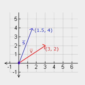
Below you can see 3 vectors, each of which is represented as (x, y) as arrows on a 2D graph. Since it is more intuitive to represent vectors in 2D (than in 3D), then you can think of 2D vectors as 3D vectors, but with a zero z coordinate. As long as the vector describes the direction, the position of the vector does not change its value. On the graph you can see that the vectors v and w are the same, although the positions differ:

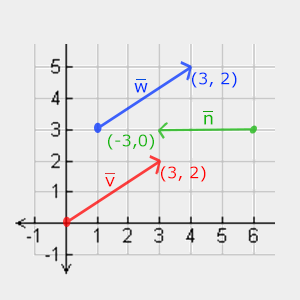
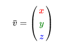
When mathematicians describe vectors, they prefer to use lower case letters with a small dash on top. Example:

Since vectors often describe a direction, sometimes they are hard to imagine as a position. Usually we visualize the vector as follows: we set the center to (0, 0, 0) , and then indicate the direction described by the point. Thus, a positional vector is obtained (we can also take another point as the center, and then say “This vector points to a point in space from this point”). The positional vector (3, 5) will point to the point (3, 5) on the graph with the base (0, 0) . With the help of vectors, we can describe both directions and positions in two-dimensional and three-dimensional spaces.

We can also perform some mathematical operations on vectors.

Scalar vector operations

A scalar is a single number (or a one-component vector if you want to continue working with vectors). When adding / subtracting / multiplying or dividing a vector by a scalar, we simply add / subtract / multiply or divide each element of the vector by this scalar. Example:

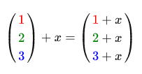
Where instead of addition there can be subtraction, multiplication or division.

Reverse vector

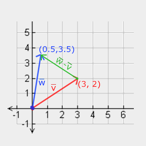
The inversion (negation) of a vector is the receipt of a vector whose direction is opposite to the original one. The reverse vector for the vector pointing to the northeast will be the vector pointing to the southwest. To reverse the vector, we simply multiply the vector by -1. Example:

Addition and subtraction

The addition of two vectors is done componentwise . Example:

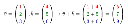
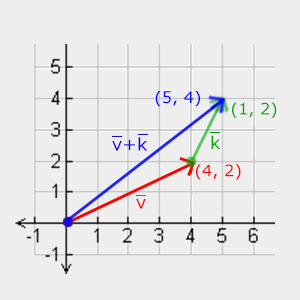
Visually, the sum of the vectors v = (4,2) and k = (1,2) looks like this:

As with ordinary addition and subtraction, the subtraction of vectors is also an addition, but with the inverse second vector:

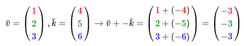
Subtracting vectors from each other generates a vector, which is the difference in the positions of the operands:

Length

To obtain the length (modulus) of a vector, we use the Pythagorean theorem , which you may remember from school. A vector forms a triangle if you present its components as the sides of a triangle:

Since the length of the sides (x, y) is known, and we want to know the length of the hypotenuse, then we do it as follows:

Where || v || Is the length of the vector v . Such a formula is easily expanded in 3D by adding z ^ 2 . Length calculation example:

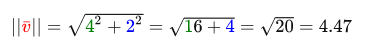
Calculated value: 4.47

There is also a special kind of vectors called unit vectors . A feature of such vectors is that their length is always equal to 1. We can convert any vector into a unit by dividing this vector by its length:

Such a vector is called normalized . Unit vectors are denoted with a small roof above the letter. It is also easier to work with them, since we only have to take care of the direction of such a vector.

Vector multiplication by vector

The multiplication of two vectors is rather strange. Normal multiplication is not applicable because it has no visual meaning, but we have 2 specific approaches from which to choose during multiplication: the first is a scalar product, which is depicted as a point, and the second is a vector product, which is depicted as a cross.

Scalar product

The scalar product of two vectors is equivalent to the scalar product of the lengths of these vectors multiplied by the cosine of the angle between them. If this sentence confuses you, then look at the formula:

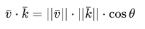
Where the angle between the vectors is described as theta . Why can this be interesting? Well, imagine if the vectors v and k are unit vectors. Accordingly, the formula is reduced to:

Now the dot product defines only the angle between the two vectors. You may remember that the cos function becomes 0, with an angle of 90 degrees and 1 with an angle of 0. This makes it easy to check whether the vectors are orthogonal or parallel to each other (orthogonality means that the vectors are rectangular). If you want to learn more about sin or cosine , then I recommend the Khan Academy video about basic trigonometry.

You can also calculate the angle between two non-unit vectors, but for this you have to divide the result by the lengths of these vectors in order to stay with cos only.

So how to count the scalar product? Scalar product is the multiplication of the components of the vectors and the subsequent addition of the results. Example:

To calculate the angle between the vectors, we need to invert the cosine function (cos ^ -1) in this case - it is 143.1 degrees. Thus, we effectively calculated the angle between these two vectors. Scalar work is very useful when working with light.

Vector product

A vector product is possible only in three-dimensional space and takes two non-parallel vectors as input, and returns a vector that is orthogonal to the input. If the input vectors are orthogonal to each other, then the vector product will create 3 orthogonal vectors. Next, you will learn why this may be useful. The following image shows how this looks like three-dimensional space:

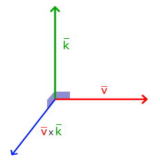
Unlike other operations, the vector product is not very intuitive without going into linear algebra, so it’s best to just remember the formula. The following is a vector product between two orthogonal vectors A and B.

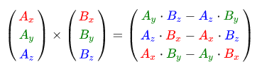
As you can see, there is not much meaning in this formula. In any case, after all these steps, you get a vector that will be orthogonal to the input.

Matrices

Now, after we have discussed almost everything about vectors, it is time to delve into the matrices. A matrix is ​​usually quadrangles from a set of numbers, symbols, and / or expressions. Here is an example of a 2x3 matrix:

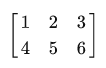
The elements of the matrix are accessed using (i, j) , where i is a row and j is a column. That is why the matrix above is called 2x3 (3 columns and 2 rows). Such a system is the opposite of that used in 2D graphs (x, y) . To obtain the value of 4 from the matrix above, we must specify the index (2, 1) (second row, first column).

Matrices, in fact, are nothing more than quadrangular arrays of mathematical expressions. They also have a very nice set of mathematical properties and, like the vectors, have several operations - addition, subtraction and multiplication.

Addition and subtraction

The addition of the matrix with a scalar is performed as follows:

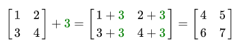
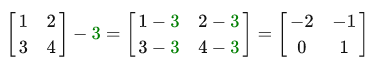
The scalar is simply added throughout the elements of the matrix. The same thing happens when subtracting:

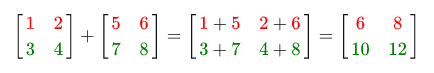
Addition and subtraction between two matrices is performed elementwise. Thus, addition and subtraction operations can only be applied to matrices of the same size. Example:

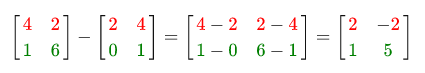
Same as with subtraction:

Matrix multiplication by scalar

As well as addition and subtraction, the matrix is ​​multiplied by a scalar by multiplying each element of the matrix by a scalar. Example:

Matrix multiplication

Matrix multiplication is not very difficult, but not so simple. Multiplication has several limitations:

1. You can only multiply matrices, where the number of columns of the first matches the number of rows of the second matrix.
2. Matrix multiplication is not commutative. A * B! = B * A.

Here is an example of multiplying two 2x2 matrices:

Now, maybe you are trying to understand what is going on here? Matrix multiplication is a combination of normal multiplication and addition using the rows of the left matrix with the columns of the right matrix. The following image should bring some clarity:

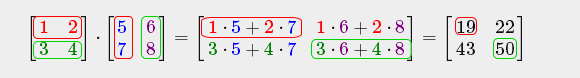
In the beginning we take the top row of the left matrix and the left column of the right matrix. The row and column we choose determines which element of the resulting matrix we are going to calculate. If we took the first row of the left matrix, then we are going to work with the top row of the resulting matrix, then we select the column in the right matrix, it determines which column of the resulting matrix we are working with. To calculate the bottom-right element, we must select the bottom row of the left matrix and the right column of the right matrix.

To calculate the resulting value, we multiply the elements of the row and column using ordinary multiplication. The results of the multiplication are then added up and we get the result. This is where the first limit comes from.

The result is a matrix of size (n, m) , where n is the number of rows in the left matrix, and m is the number of columns in the right matrix.

If you have a problem - do not worry. Just keep on calculating with your hands and return to this lesson when difficulties arise. Soon the multiplication of matrices will be on the machine.

Let's close the matrix multiplication question with one big example. For the presentation of the algorithm used colors. For training, try to calculate the result yourself, and then compare it with the result in the example.

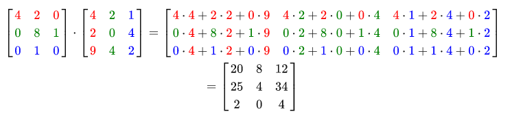
As you can see the multiplication of matrices is a rather dreary process with a lot of places to go wrong. And these problems only grow with increasing size. If you are still craving more mathematical properties of matrices, I highly recommend the Khan Academy video .

Matrix vector multiplication

We have already used vectors in past lessons. We used them to represent positions, colors, and texture coordinates. Now let's dive a little into the rabbit hole and tell you that the vector is actually just an Nx1 matrix, where N is the number of components of the vector. If you think about it a little, it makes sense. The vectors, just like matrices, are an array of numbers, but only with 1 column. And how will this information help us? Well, if we have an MxN matrix, we can multiply it by the Nx1 vector, since the number of columns of the matrix is ​​equal to the number of rows of the vector.

But why should we even be able to multiply the matrix by the vector? Quite a lot of different 3D / 2D transformations can be performed by multiplying the matrix by a vector, obtaining a modified vector. If you are still not sure that you fully understand the text above, here are some examples:

Unit matrix

In OpenGL, they usually work with 4x4 transformation matrices for the reason that most vectors have 4 components. The simplest transformation matrix that can be discussed is the identity matrix . The identity matrix is ​​an NxN matrix, filled with zeros, but with 1 diagonally. As we can see, this matrix does not change the vector at all:

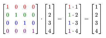
Vector looks intact. This becomes obvious from the multiplication rules: the first resultant element is each element of the first row of the matrix, multiplied by each element of the vector. Since each element of the line is 0, except for the first one, we get 1 * 1 + 0 * 2 + 0 * 3 + 0 * 4 = 1. The same applies to the remaining 3 elements of the vector.

You may ask, why would a transformation matrix, which transforms nothing, be needed at all? The identity matrix is ​​often the starting point for generating other transformation matrices and if we delve into linear algebra, this is also a very convenient matrix for proving theorems and solving linear equations.

Scaling matrix

When we scale a vector, we increase the length of the arrow by the amount of scaling, keeping the direction. While we are working in 2 or 3 dimensions, we can define a vector scaling of 2 or 3 values, each of which scales one of the axes (x, y or z) .

Let's try to scale the vector v = (3,2) . We will scale the vector along the x axis by 0.5 , which will make it 2 times narrower; and scale the vector along the y axis by 2 , which will increase the height by 2 times. Let's see how it will look like if we scale the vector by (0.5, 2). We write the result as s .

Remember that OpenGL often works in 3D space, so for 2D you can leave the Z coordinate equal to 1. The scaling operation that we just performed is non-uniform , since the scaling value for each axis is different. If the scaling value were the same, then such a transformation is called homogeneous .

Let's build a transformation matrix that will scale for us. We have already seen on the identity matrix that the diagonal element will be multiplied by the corresponding element of the vector. What if we replace the units in the unit matrix for triples? In this case, we multiply all elements of the vector by this value. Accordingly, if we represent the scaling values ​​as (S1, S2, S3), then we will be able to determine the scaling matrix for any vector (x, y, z) :

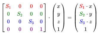
Note that the 4th element of the vector is 1. This component is denoted as w and will later be used for other tasks.

Shear matrix

Shift is the process of adding one vector to another to obtain a new vector with a different position, that is, a vector shift based on a shift vector. We have already discussed vector addition, so for you this will not be something new.
As with the scaling matrix in the 4x4 matrix there are several positions for performing the required operations, for shifting these are the top 3 elements of the fourth column. If we represent the shift vector as (Tx, Ty, Tz), then we can define the shift matrix as follows:

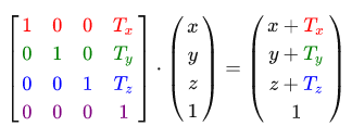
This works because all the values ​​of the vector are multiplied by the w components of the vector and added to the initial values. This would not be possible using 3x3 matrices.

Homogeneous coordinates
The component of the vector w is also called a homogeneous coordinate . To obtain a 3D vector from a homogeneous coordinate, we divide the x , y, and z coordinates by w . This is usually not noticed, since w is most of the time 1.0. Using homogeneous coordinates has several advantages: they allow us to perform shifts on 3D vectors (without the w components, this would be impossible) and in the next chapter we will use the value of w to create 3D visualizations.
Also, when the homogeneous coordinate is 0, then the vector is considered to be a direction vector , since the vector with the w component equal to 0 cannot be shifted.

With the shift matrix, we can move objects in all 3 directions (x, y, z) , which makes this matrix extremely useful for our tasks.

Rotation matrix

The last couple of transformations were fairly easy to understand and view in 2D or 3D space, but the rotations are a bit more intricate. If you want to know how exactly these matrices are formed - then I recommend the Khan Academy video about linear algebra .

To begin with, let's define what this is - rotation of a vector. Rotation in 2D and 3D is determined by the angle . The angle can be expressed in angles or radians, in which a full revolution is 360 degrees or 2Pi, respectively. I prefer to work with degrees, since they are more logical for me.

Most rotational functions require an angle in radians, but the benefit of converting from one system to another is quite simple:
Degrees = radians * (180.0f / PI)
Radians = degrees * (PI / 180.0f)
Where PI is approximately 3.14159265359

Rotation on a half circle - requires us to rotate 360/2 = 180 degrees. Rotation 1/5 to the right requires us to rotate 360/5 = 72 degrees to the right. Here is an example of a conventional 2D vector, where v is rotated 72 degrees to the right of k .

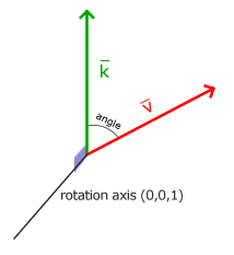
Rotation in 3D is described by the angle and axis of rotation . The angle determines how much the vector will be rotated about the given axis. When rotating 2D vectors in the 3D world, for example, we set the rotation axis - Z.

With the help of trigonometry, we can transform vectors into rotated at a certain angle. This is usually done with a clever combination of sin and cos functions. A discussion of how the transformation matrix is ​​generated is beyond the scope of our lesson.

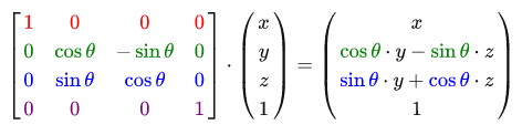
The rotation matrix is ​​defined for each axis in 3D space, where the angle is shown as theta.
Rotation matrix around the X axis:

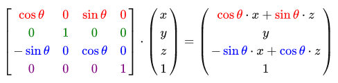
The rotation matrix around the Y axis:

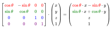
The rotation matrix around the Z axis:

With the help of rotation matrices, we can rotate our vectors along one of three axes. You can also combine them, for example, at the beginning turn on the X axis, and then Y. True, this approach will quickly lead to a problem called the hinge lock problem. We will not go into details, but it is better to use rotation along a specific axis, for example (0.662, 0.2, 0.722) (note that this is a single vector), instead of combining rotation along specific axes. The matrix for such transformations exists and looks like this, where (Rx, Ry, Rz) is the axis of rotation:

Mathematical discussions about generating such a matrix are beyond the scope of this lesson. Just keep in mind that even such a matrix does not completely solve the problem of the hinge lock (it's just harder to get). In order to completely solve this problem, we will have to work with rotations using quaternions, which are not only safer, but also much more friendly from the point of view of calculations. Be that as it may, the Quaternion discussion is set aside for a later lesson.

Matrix Combination

In order to maximize the utility of using matrices for transformations, we need to combine transformation matrices into one matrix. Let's see if we can generate a transformation matrix that will include several transformations. For example, we have a vector (x, y, z) and we want to scale it 2 times and shift by (1, 2, 3) . To do this, we need scaling and offset matrices. As a result, we get something like:

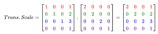
Notice that during the multiplication of matrices, we first perform a shift, and then scaling. Matrix multiplication is not commutative, which means that the order of multiplication is important. During matrix multiplication, the right matrix is ​​multiplied by a vector, so you need to read the multiplications from right to left. It is recommended to scale at the beginning, then rotate and shift at the end, during the union of the matrices, otherwise they can deny each other. For example, if you first shift and then scale, then the shift matrix will also scale!

As a result, the transformation matrix is ​​applied as follows:

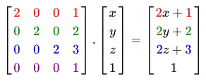
Excellent, the vector is scaled 2 times and shifted by (1, 2, 3) .

On practice

After we discussed the whole theory, it is time to put it into practice. OpenGL does not have built-in support for matrix or vector transformations, so we will have to use our own math classes and functions. In these lessons we abstract from subtle mathematical details and simply use ready-made mathematical libraries. Fortunately, there is already an easy-to-use and sharpened math library called OpenGL called GLM.

GLM

GLM is an abbreviation for Open GL M athematics. This library is a header, which means that we just need to include the required header files. No need to bother with any linking or compilation. GLM can be downloaded from the official site . Copy the root directory with the header files to your includes folder and you can start.

Most of the GLM functionality can be found in the 3 header files:

#include <glm/glm.hpp> #include <glm/gtc/matrix_transform.hpp> #include <glm/gtc/type_ptr.hpp> 

Let's see if we can apply our knowledge in the transformations to shift the vector (1, 0, 0) to (1, 1, 0) (note that we denoted from glm :: vec4 with a homogeneous coordinate of 1.0):

 glm::vec4 vec(1.0f, 0.0f, 0.0f, 1.0f); glm::mat4 trans; trans = glm::translate(trans, glm::vec3(1.0f, 1.0f, 0.0f)); vec = trans * vec; std::cout << vec.x << vec.y << vec.z << std::endl; 

In the beginning, we created a vector called vec using the built-in GLM vector class. Then we define mat4 , which is the 4x4 identity matrix. Then we create the transformation matrix by passing our unit matrix to the function glm :: translate , along with the shift vector.
Then we multiply our vector by the transformation matrix and output the result. If you still remember how the shift matrix works, then you understand that the resulting vector must be (1 + 1, 0 + 1, 0 + 0) , which is (2, 1, 0) . The code above displays 210 , which means that the shift matrix has done its job.

Let's try to do something more interesting and try to scale and then rotate an object from the last lesson. At the beginning we will rotate the container 90 degrees counterclockwise. Then scale it to 0.5 in order to reduce it by 2 times. Let's build a transformation matrix for this.

 glm::mat4 trans; trans = glm::rotate(trans, 90.0f, glm::vec3(0.0, 0.0, 1.0)); trans = glm::scale(trans, glm::vec3(0.5, 0.5, 0.5)); 

At the beginning, we reduce the container by 0.5, along each axis, and then rotate the container 90 degrees in the Z coordinate. Notice that the texture also turned. Since we pass the matrix to each of the GLM functions, GLM automatically multiplies the matrices, resulting in a transformation matrix.

Some versions of GLM take angles in radians, not degrees. If you have such a version, convert the degrees to radians using glm :: radians (90.0f) .

The next big question is how to pass the transformation matrix to the shader? We have already said that GLSL is of type mat4 . So it remains for us to accept mat4 as the uniform variable and multiply the position vector by this matrix.

 #version 330 core layout (location = 0) in vec3 position; layout (location = 1) in vec3 color; layout (location = 2) in vec2 texCoord; out vec3 ourColor; out vec2 TexCoord; uniform mat4 transform; void main() { gl_Position = transform * vec4(position, 1.0f); ourColor = color; TexCoord = vec2(texCoord.x, 1.0 - texCoord.y); } 

GLSL also has mat2 and mat3 types , which provide the same operations as vectors. All operations covered in this article are available in matrix types.

We added uniform and multiplied the positional vector by the transformation matrix before passing it to gl_Position . Our container should now be less than 2 times and turn 90 degrees. But do we still need to pass the transformation matrix to the shader?

 GLuint transformLoc = glGetUniformLocation(ourShader.Program, "transform"); glUniformMatrix4fv(transformLoc, 1, GL_FALSE, glm::value_ptr(trans)); 

At the beginning we get the position of the uniform variable and then send the matrix data to it using the glUniform function with the postfix Matrix4fv . The first argument must be a variable position. The second argument tells OpenGL how many matrices we are going to send, in our case 1. The third argument tells you if you want to transpose the matrix. OpenGL developers often use an internal matrix format called column-major ordering, which GLM uses by default, so we do not need to transpose the matrices, we can leave GL_FALSE . The last parameter is the data itself, but GLM does not store the data exactly as OpenGL wants to see it, so we convert it using value_ptr .

We created a transformation matrix, declared uniform in the vertex shader, and sent the matrix in the shader with which we adjust the vertex coordinates. The result should be something like this:

Fine! Our container is really turned left and 2 times smaller, so the transformation was successful. And now let's make our container rotate in real time, and also move it to the lower right corner. In order to do this, you will have to perform calculations at each iteration of the main loop. We use the GLFW function to get time to change the angle over time:

 glm::mat4 trans; trans = glm::translate(trans, glm::vec3(0.5f, -0.5f, 0.0f)); trans = glm::rotate(trans,(GLfloat)glfwGetTime() * 50.0f, glm::vec3(0.0f, 0.0f, 1.0f)); 

Keep in mind that earlier we could declare a transformation matrix anywhere, but now we create it at each iteration so that we can update the rotation for each frame. This means that we must recreate the transformation matrix at each iteration of the game cycle. Usually, when there are several objects on stage, their transformation matrices are recreated with new values ​​at each iteration of the drawing.

Now we rotate the object around the center (0, 0, 0) , and then move the rotated version to the bottom-right corner of the screen. Remember that the real sequence of applying transformations is read in the reverse order: even in the code we shift at the beginning and then rotate, then the transformations are applied in the reverse order, at the beginning of the turn, then the shift. Understanding all these transformations and how they affect objects is rather difficult. Try experimenting with transformations and get used to them quickly.

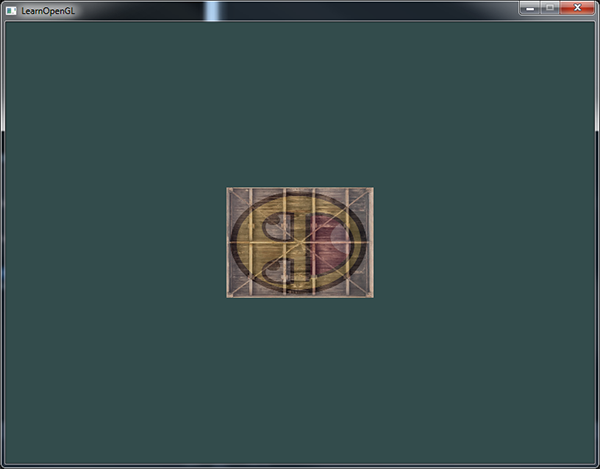
If you did everything right, then you get something like this:

That's all. A shifted container that rotates over time, and all this is done with a single transformation matrix! Now you can see why matrices are so strong in the graphic world. We can define an infinite number of transformations and combine them into one matrix for subsequent reuse. Using such transformations in the vertex shader allows us not to change the vertex data, which saves us processor time, since we do not need to send data to the buffer.

If you could not get the correct result or you are stuck somewhere, then take a look at the source code together with the vertex and fragment shaders.

In the next lesson, we will discuss how to use matrices to define different coordinate spaces for our vertices. This will be a new step in the world of 3D graphics in real time!

Exercises

• Change the last transformation of the sequence of actions, see what happens, try to justify why this is the result. Decision
• Try drawing another container with glDrawElements , but just place the container in a different place with a different transformation. Let it be in the upper right corner and instead of rotating - it changed its size (here you can use the sin function): Solution