Neural network optimization methods

In the overwhelming majority of sources of information about neural networks, “now let's educate our network” means “feed the objective function to the optimizer” with only the minimum learning speed setting. It is sometimes said that the weights of the network can be updated not only by stochastic gradient descent, but without any explanation what the other algorithms are notable for and what the mysterious ones mean $\ inline \ beta$ and $\ inline \ gamma$ in their parameters. Even teachers in machine learning courses often do not focus on this. I would like to correct the lack of information in runet about various optimizers that you may encounter in modern machine learning packages . I hope my article will be useful to people who want to deepen their understanding of machine learning or even invent something of their own.

Under the cut a lot of pictures, including animated gif.

The article is aimed at a reader familiar with neural networks. It is assumed that you already understand the essence of backpropagation and SGD . I will not go into a rigorous proof of the convergence of the algorithms presented below, but on the contrary, I will try to convey their ideas in simple language and show that the formulas are open for further experiments. The article lists not all the complexities of machine learning and not all the ways to overcome them.

Why do we need tricks

Let me remind you what formulas look like for ordinary gradient descent:

$\ Delta \ theta = - \ eta \ nabla_ \ theta J (\ theta)$

$\ theta = \ theta + \ Delta \ theta = \ theta - \ eta \ nabla_ \ theta J (\ theta)$

Where $\ inline \ theta$ - network settings $\ inline J (\ theta)$ - the objective function or loss function in the case of machine learning, and $\ inline \ eta$ - learning speed. It looks amazingly simple, but a lot of the magic is hidden in $\ inline \ nabla_ \ theta J (\ theta)$ - update the parameters of the output layer is quite simple, but to get to the parameters of the layers behind it, you have to go through nonlinearities, the derivatives of which contribute to. This is the familiar principle of the reverse propagation of error - backpropagation.

Explicitly written formulas for updating the scales somewhere in the middle of the network look ugly, because each neuron depends on all the neurons with which it is connected, and those from all the neurons with which they are connected, and so on. At the same time, even in “toy” neural networks, there can be about 10 layers, and among the networks that keep modern classifications of modern datasets - much, much more. Each weight is variable in $\ inline J (\ theta)$ . Such an incredible amount of degrees of freedom allows you to build very complex mappings, but brings researchers a headache:

Jam at local minima or saddle points, which for a function of $\ inline & gt; 10 ^ 6$ There may be a lot of variables.
The complex landscape of the objective function: the plateau alternates with regions of strong nonlinearity. The derivative on the plateau is almost zero, and a sudden break, on the contrary, can send us too far.
Some parameters are updated much less frequently than others, especially when there are informative, but rare signs in the data, which have a bad effect on the nuances of the generalizing network rule. On the other hand, giving too much importance to all rarely encountered symptoms in general can lead to retraining.
Too small learning rate makes the algorithm converge for a very long time and get stuck in local minima, too large - to “fly” narrow global minima or to completely diverge

Computational mathematics known advanced algorithms of the second order, which is able to find a good minimum and on a complex landscape, but then the amount of weights hits again. To use the honest method of the second order "in the forehead," you will have to calculate the Hessian $\ inline J (\ theta)$ - the matrix of derivatives for each pair of parameters of a pair of parameters (already bad) - and, say, for the Newton method, also the inverse of it. We have to invent all sorts of tricks to cope with the problems, leaving the task of computationally lifting. Second-order working optimizers exist , but for now let's concentrate on what we can achieve without considering the second derivatives.

Nesterov Accelerated Gradient

By itself, the idea of methods with the accumulation of momentum is obviously simple: "If we move for a while in a certain direction, then we probably should go there for some time in the future." To do this, you need to be able to refer to the recent change history of each parameter. You can store the latest $\ inline n$ copies $\ inline \ Delta \ theta$ and at each step it is fair to assume an average, but this approach takes too much memory for large $\ inline n$ . Fortunately, we do not need an exact average, but only an estimate, so we use an exponential moving average.

$v_t = \ gamma v_ {t-1} + (1- \ gamma) x$

To accumulate something, we will multiply the accumulated value by the conservation factor $\ inline 0 & lt; \ gamma & lt; one$ and add another value multiplied by $\ inline 1- \ gamma$ . The closer $\ inline \ gamma$ to one, the larger the accumulation window and the stronger the smoothing is history $\ inline x$ begins to influence more than every next $\ inline x$ . If a $\ inline x = 0$ from a certain moment $\ inline v_t$ decay exponentially exponentially, hence the name. We apply the exponential running average to accumulate the gradient of the objective function of our network:

$v_t = \ gamma v_ {t-1} + \ eta \ nabla_ \ theta J (\ theta)$

$\ theta = \ theta - v_t$

Where $\ inline \ gamma$ usually takes order $\ inline 0.9$ . note that $\ inline 1- \ gamma$ not lost, but included in $\ inline \ eta$ ; Sometimes you can find a variant of the formula with an explicit multiplier. The smaller $\ inline \ gamma$ , the more the algorithm behaves like a normal SGD. To get a popular physical interpretation of the equations, imagine a ball rolling on a hilly surface. If at the moment $\ inline t$ under the ball there was a nonzero bias ( $\ inline \ nabla_ \ theta J (\ theta)$ ), and then he hit the plateau, he will continue to roll on this plateau anyway. Moreover, the ball will continue to move a couple of updates in the same direction, even if the bias has changed to the opposite. However, viscous friction acts on the ball and every second it loses $\ inline 1- \ gamma$ its speed. Here is what the accumulated impulse looks like for different $\ inline \ gamma$ (hereinafter, epochs are plotted along the X axis, and the gradient value and the accumulated values are along the Y axis):

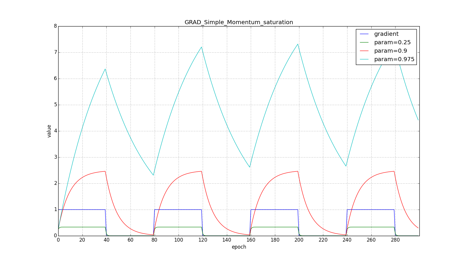
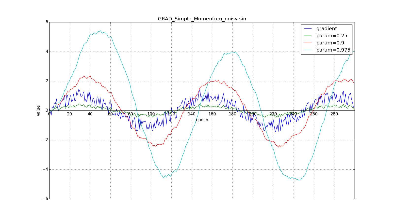
Note that the accumulated in $\ inline v_t$ the value can greatly exceed the value of each of $\ inline \ eta \ nabla_ \ theta J (\ theta)$ . A simple accumulation of momentum already gives a good result, but Nesterov goes further and applies the well-known idea in computational mathematics: looking ahead along the update vector. Since we're still going to shift to $\ inline \ gamma v_ {t-1}$ then let's calculate the loss function gradient not at the point $\ inline \ theta$ and in $\ inline \ theta - \ gamma v_ {t-1}$ . From here:

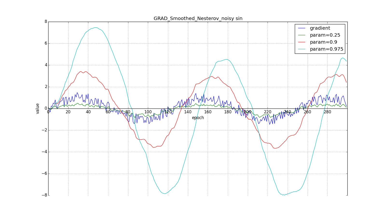
$v_t = \ gamma v_ {t-1} + \ eta \ nabla_ \ theta J (\ theta - \ gamma v_ {t-1})$

$\ theta = \ theta - v_t$

Such a change allows you to “roll” faster if, aside, where we are going, the derivative increases, and more slowly, if vice versa. This is especially evident for $\ inline \ gamma = 0.975$ for a graph with a sine.

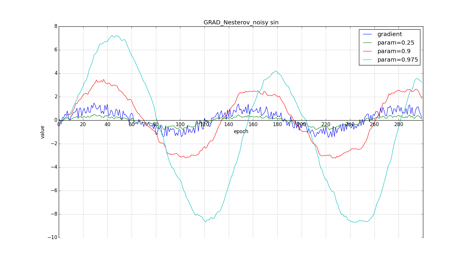
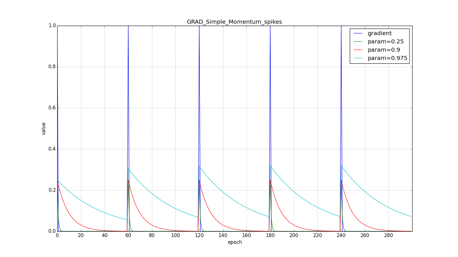
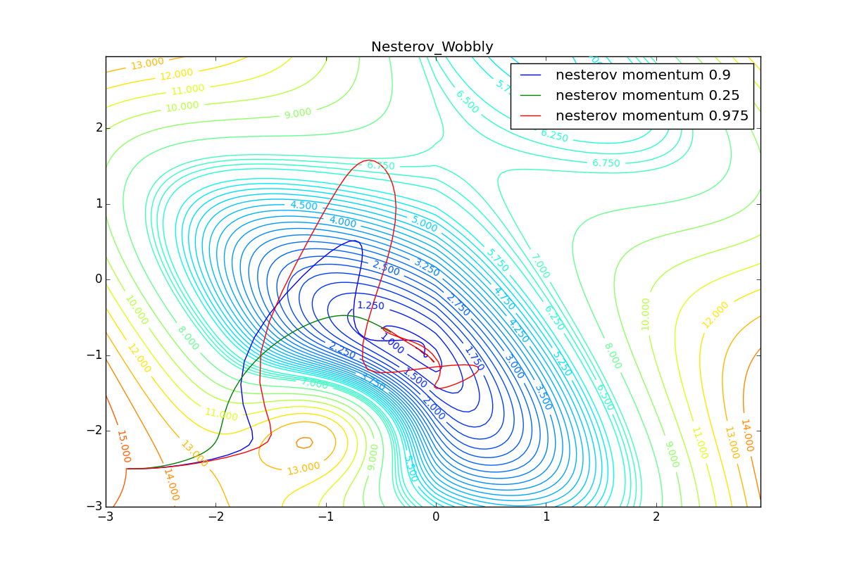
Looking ahead can play a cruel joke on us if you set too large $\ inline \ gamma$ and $\ inline \ eta$ : we look so far as to miss the areas with the opposite gradient sign:

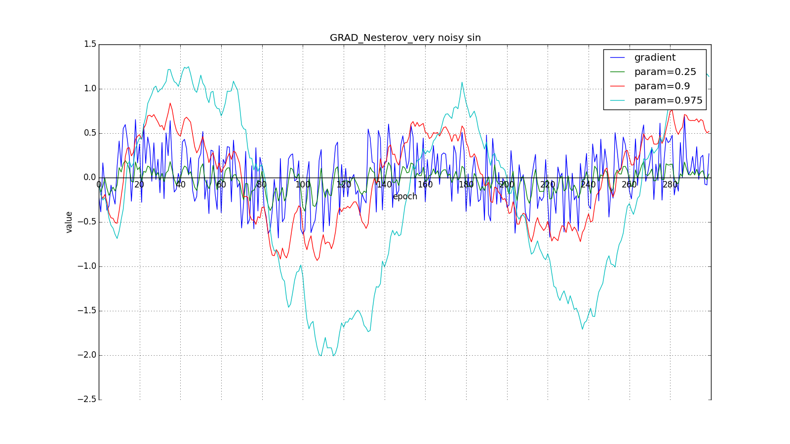
However, sometimes this behavior may be desirable. Once again I draw your attention to the idea - looking ahead - and not to execution. Nesterov's method (6) is the most obvious option, but not the only one. For example, you can use another technique from computational mathematics — stabilization of the gradient by averaging over several points along the line along which we move. So to speak:

$v_t = \ gamma v_ {t-1} + \ frac {\ eta} {3} \ big (\ nabla_ \ theta J (\ theta - \ frac {\ gamma v_ {t-1}} {3}) + \ nabla_ \ theta J (\ theta - \ frac {2 \ gamma v_ {t-1}} {3}) + \ nabla_ \ theta J (\ theta - \ gamma v_ {t-1}) \ big)$

Or so:

$v_t = \ gamma v_ {t-1} + \ frac {\ eta} {7} \ big (\ nabla_ \ theta J (\ theta - \ frac {\ gamma v_ {t-1}} {2}) + 2 \ nabla_ \ theta J (\ theta - \ frac {3 \ gamma v_ {t-1}} {4}) + 4 \ nabla_ \ theta J (\ theta - \ gamma v_ {t-1}) \ big)$

Such a technique can help in the case of noisy target functions.

We will not manipulate the argument of the objective function in the subsequent methods (although, of course, no one bothers to experiment). Further, for brevity

$g_t \ equiv \ nabla_ \ theta J (\ theta_t)$

Adagrad

How many methods work with the accumulation of momentum Let us turn to more interesting optimization algorithms. Let's start with a relatively simple Adagrad - adaptive gradient.

Some signs may be extremely informative, but rarely occur. Exotic high-paying profession, a fancy word in the spam database - they will easily drown in the noise of all other updates. It is not only about rarely encountered input parameters. Say, you may well encounter rare graphic patterns that even become a sign only after passing through several layers of a convolutional network. It would be nice to be able to update the parameters with an eye on how typical they sign. To achieve this is not difficult: let's store for each network parameter the sum of the squares of its updates. It will act as a proxy for typicality: if the parameter belongs to a chain of frequently activated neurons, it is constantly pulled back and forth, which means the amount quickly accumulates. Rewrite the update formula like this:

$G_ {t} = G_ {t} + g_ {t} ^ 2$

$\ theta_ {t + 1} = \ theta_ {t} - \ frac {\ eta} {\ sqrt {G_ {t} + \ epsilon}} g_ {t}$

Where $\ inline G_ {t}$ - the sum of the squares of the updates, and $\ inline \ epsilon$ - smoothing parameter necessary to avoid dividing by 0. The parameter that was frequently updated in the past is large $\ inline G_t$ , is the big denominator in (12). Parameter changed only one or two will be updated in full force. $\ inline \ epsilon$ take order $\ inline 10 ^ {- 6}$ or $\ inline 10 ^ {- 8}$ for a completely aggressive update, but, as can be seen from the graphs, this plays a role only at the beginning, towards the middle, the training begins to outweigh $\ inline G_t$ :

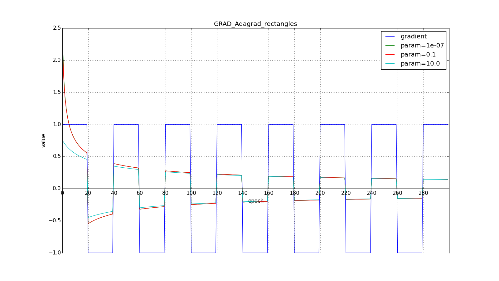
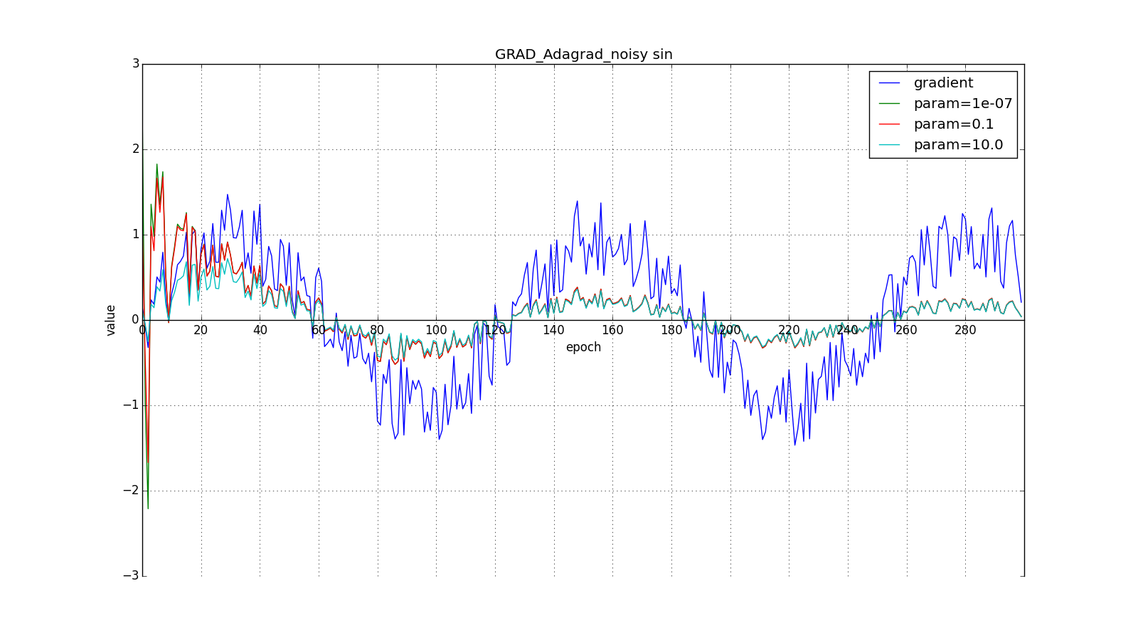
So, the idea of Adagrad is to use something that would reduce updates for the elements that we update so often. Nobody forces us to use this particular formula, therefore Adagrad is sometimes called a family of algorithms. Let's say we can remove the root or accumulate not the squares of updates, but their modules, or even replace the multiplier with something like $\ inline e ^ {- G_ {t}}$ .

(Another thing is that this requires experimentation. If you remove the root, updates will start to decrease too quickly, and the algorithm will get worse)

Another advantage of Adagrad is the absence of the need to accurately select the speed of learning. It is enough to set it moderately large to provide a good margin, but not so huge that the algorithm diverges. In fact, we automatically get the decay rate of learning (learning rate decay).

RMSProp and Adadelta

The disadvantage of Adagrad is that $\ inline G_ {t}$ in (12) it can increase as much as necessary, which after a while leads to too small updates and paralysis of the algorithm. RMSProp and Adadelta are designed to correct this flaw.

Modifying the idea of Adagrad: we are still going to update less weight, which are updated too often, but instead of the total amount of updates, we will use the history-averaged square of the gradient. Again we use the exponentially decaying running average.
(four). Let be $\ inline E [g ^ 2] _t$ - running average at the moment $\ inline t$

$E [g ^ 2] _t = \ gamma E [g ^ 2] _ {t-1} + (1 - \ gamma) g ^ 2_t$

then instead of (12) we get

$\ theta_ {t + 1} = \ theta_ {t} - \ frac {\ eta} {\ sqrt {E [g ^ 2] _t + \ epsilon}} g_ {t}$

The denominator is the root of the mean squares of the gradients, hence RMSProp - root mean square propagation

$RMS [g] _t = \ sqrt {E [g ^ 2] _t + \ epsilon}$

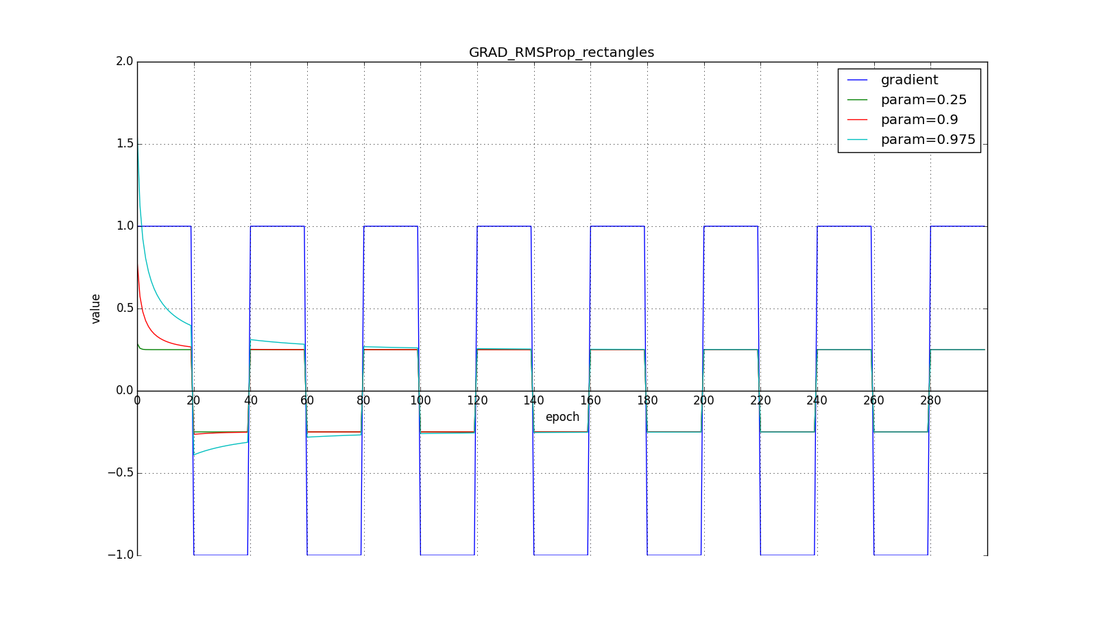
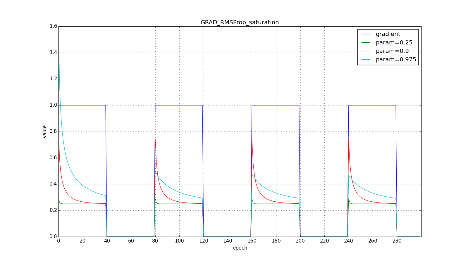
Notice how the refresh rate is restored on the chart with long teeth for different $\ inline \ gamma$ . Also compare the graphs with the meander for Adagrad and RMSProp: in the first case, the updates are reduced to zero, and in the second - they reach a certain level.

That's the whole RMSProp. Adadelta differs from it in that we add to the numerator (14) the stabilizing term proportional $\ inline RMS$ from $\ inline \ Delta \ theta_t$ . On the move $\ inline t$ we don't know the meaning yet $\ inline RMS [\ Delta \ theta] _ {t}$ therefore, the parameters are updated in three stages, not two: we first accumulate the square of the gradient, then update $\ inline \ theta$ after which we update $\ inline RMS [\ Delta \ theta]$ .

$\ Delta \ theta = - \ frac {RMS [\ Delta \ theta] _ {t-1}} {RMS [g] _ {t}} g_ {t}$

$\ theta_ {t + 1} = \ theta_ {t} - \ frac {RMS [\ Delta \ theta] _ {t-1}} {RMS [g] _ {t}} g_ {t}$

$E [\ Delta \ theta ^ 2] _t = \ gamma E [\ Delta \ theta ^ 2] _ {t-1} + (1 - \ gamma) \ Delta \ theta ^ 2_t$

$RMS [\ Delta \ theta] _ {t} = \ sqrt {E [\ Delta \ theta ^ 2] _t + \ epsilon}$

Such a change is made from considerations that the dimensions $\ inline \ theta$ and $\ inline \ Delta \ theta$ must match. Notice that the learning rate has no dimension, which means that in all the algorithms before that, we added the dimensional quantity with the dimensionless one. Physicists in this place will be horrified, and we shrug our shoulders: it works the same.

Note that we need a nonzero $\ inline RMS [\ Delta \ theta] _ {- 1}$ for the first step, otherwise all subsequent $\ inline \ Delta \ theta$ and therefore $\ inline RMS [\ Delta \ theta] _ {t}$ will be zero. But we solved this problem even earlier, adding to $\ inline RMS$ $\ inline \ epsilon$ . Another thing is that without an obvious big $\ inline RMS [\ Delta \ theta] _ {- 1}$ we get the opposite behavior of Adagrad and RMSProp: we will be stronger (to a certain extent) update weights that are used more often . After all, now to $\ inline \ Delta \ theta$ became significant, the parameter must accumulate a large amount in the numerator of the fraction.

Here are the graphics for the zero starting $\ inline RMS [\ Delta \ theta]$ :

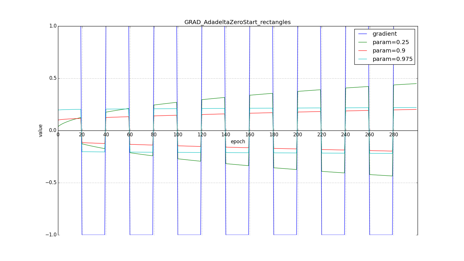
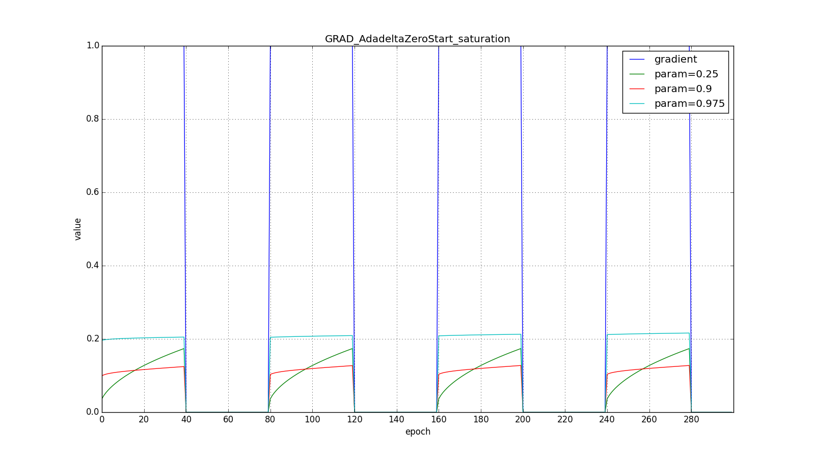
But for the big one:

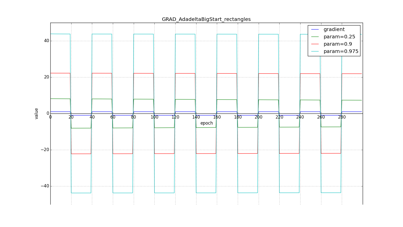
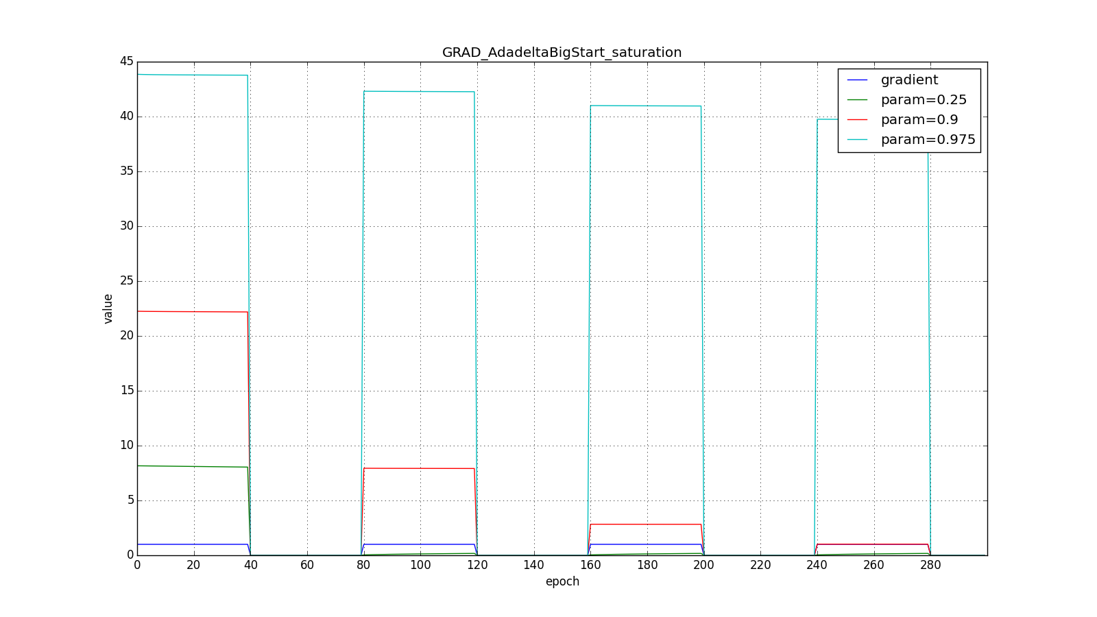
However, it seems, the authors of the algorithm and sought such an effect. For RMSProp and Adadelta, as well as for Adagrad, it is not necessary to select the learning rate very precisely - just a rough value. Usually advised to start trimming. $\ inline \ eta$ c $\ inline 0.1 - 1$ a $\ inline \ gamma$ so leave $\ inline 0.9$ . The closer $\ inline \ gamma$ to $\ inline 1$ the longer RMSProp and Adadelta with more $\ inline RMS [\ Delta \ theta] _ {- 1}$ It will greatly update the little used weight. If $\ inline \ gamma \ approx 1$ and $\ inline RMS [\ Delta \ theta] _ {- 1} = 0$ , the Adadelta will treat the rarely used weights for a long time “with distrust”. The latter can lead to paralysis of the algorithm, and can cause intentionally "greedy" behavior, when the algorithm first updates the neurons that encode the best signs.

Adam

Adam - adaptive moment estimation, one more optimization algorithm. He combines the idea of the accumulation of movement and the idea of a weaker updating of the scales for typical signs. Remember again (4):

$m_t = \ beta_1 m_ {t-1} + (1 - \ beta_1) g_t$

Adam differs from Nesterov in that we accumulate not $\ inline \ Delta \ theta$ , and gradient values, although this is a purely cosmetic change, see (23). In addition, we want to know how often the gradient changes. The authors of the algorithm proposed for this to evaluate also the average non-centered variance:

$v_t = \ beta_2 v_ {t-1} + (1 - \ beta_2) g_t ^ 2$

It is easy to notice that this is already familiar to us. $\ inline E [g ^ 2] _t$ , so in fact there is no difference from RMSProp.

An important difference is in initial calibration. $\ inline m_t$ and $\ inline v_t$ : they suffer from the same problem as $\ inline E [g ^ 2] _t$ in RMSProp: if you set a zero initial value, then they will accumulate for a long time, especially with a large accumulation window ( $\ inline 0 \ ll \ beta_1 & lt; one$ , $\ inline 0 \ ll \ beta_2 & lt; one$ ), and some initial values are two more hyperparameters. No one wants two more hyperparameters, so we artificially increase $\ inline m_t$ and $\ inline v_t$ in the first steps (approximately $\ inline 0 & lt; t & lt; ten$ for $\ inline m_t$ and $\ inline 0 & lt; t & lt; 1000$ for $\ inline v_t$ )

$\ hat {m} _t = \ frac {m_t} {1 - \ beta ^ t_1}, \; \ hat {v} _t = \ frac {v_t} {1 - \ beta ^ t_2}$

In summary, the update rule is:

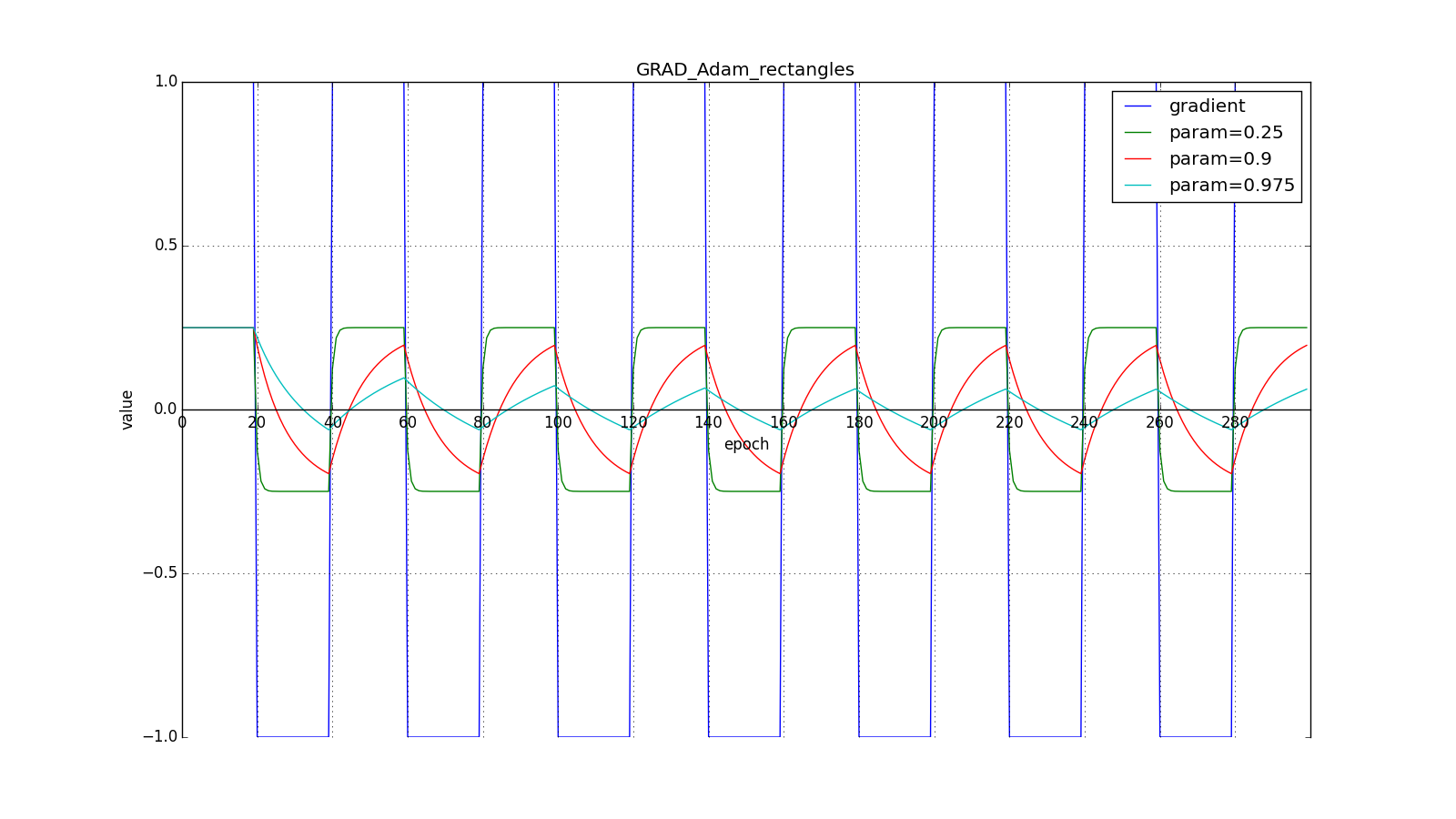
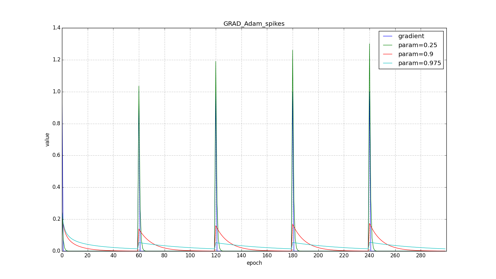
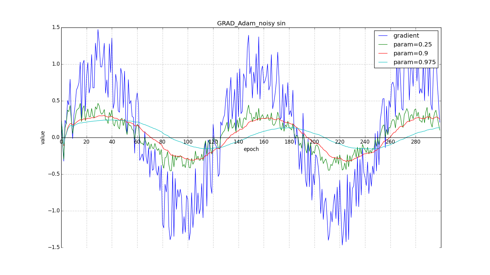
$\ theta_ {t + 1} = \ theta_ {t} - \ dfrac {\ eta} {\ sqrt {\ hat {v} _t + \ epsilon}} \ hat {m} _t$

Here you should take a close look at how quickly the values of updates synchronized on the first teeth of graphs with rectangles and on the smoothness of the update curve on a graph with a sine — we received it “for free”. With recommended setting $\ inline \ beta_1$ on the graph with spikes, it is clear that sudden gradient bursts do not cause an instantaneous response in the accumulated value, so a well-tuned Adam does not need gradient clipping.

The authors of the algorithm derive (22) by expanding the recursive formulas (20) and (21). For example, for $\ inline v_t$ :

$E [v_t] & amp; = E \ Bigg [(1 - \ beta_2) \ sum_ {i = 1} ^ {t} {\ beta_2 ^ {t-i} g_i ^ 2} \ Bigg]$

$= E [g_t ^ 2] (1 - \ beta_2) \ sum_ {i = 1} ^ {t} \ beta_2 ^ {t-i} + \ zeta$

$= E [g_t ^ 2] (1 - \ beta_2) \ frac {1 - \ beta_2 ^ t} {1 - \ beta_2} + \ zeta$

$= E [g_t ^ 2] (1 - \ beta_2 ^ t) + \ zeta$

Term $\ inline \ zeta$ close to $\ inline 0$ with stationary distribution $\ inline p (g)$ that is not true in cases practically of interest to us. but we still move the bracket with $\ inline \ beta_2 ^ t$ to the left. Informally, one can imagine that with $\ inline t = 0$ we have an endless history of identical updates:

$\ hat {v} _1 = v_ {1} + \ beta_2 v_ {1} + \ beta_2 ^ 2 v_ {1} + \ ldots = \ frac {v_ {1}} {1 - \ beta_2}$

When we get closer to the correct value $\ inline v$ , we force the “virtual” part of the series to decay faster:

$\ hat {v} _2 = v_ {2} + \ beta_2 ^ 2 v_ {2} + \ beta_2 ^ 4 v_ {2} + \ ldots = \ frac {v_ {2}} {1 - \ beta_2 ^ 2}$

Adam authors propose default values. $\ inline \ beta_1 = 0.9, \ beta_2 = 0.999, \ epsilon = 10 ^ {- 8}$ and argue that the algorithm performs better or about the same as all previous algorithms on a wide range of datasets due to the initial calibration. Notice, again, that equations (22) are not set in stone. We have some theoretical justification for why attenuation should look like this, but no one forbids experimenting with calibration formulas. In my opinion, here it is simply suggested to apply peering forward, as in the Nesterov method.

Adamax

Adamax is just such an experiment proposed in the same article. Instead of dispersion in (21), we can assume the inertial moment of the distribution of gradients of arbitrary $\ inline p$ . This can lead to instability to the calculations. However the case $\ inline p$ tending to infinity works surprisingly well.

$v_t = \ beta_2 ^ p v_ {t-1} + (1 - \ beta_2 ^ p) | g_t | ^ p$

Notice that instead $\ inline \ beta_2$ using the appropriate dimension $\ inline \ beta_2 ^ p$ . In addition, note that to use in the Adam formulas the value obtained in (27), you need to extract the root from it: $\ inline u_t = v_t ^ {\ frac {1} {p}}$ . We derive a decisive rule in return (21), taking $\ inline p \ rightarrow \ infty$ by unfolding under the root $\ inline v_t$ with the help of (27):

$u_t = \ lim_ {p \ rightarrow \ infty} {v_t ^ {\ frac {1} {p}}}$

$= \ lim_ {p \ rightarrow \ infty} {\ Big [\ beta_2 ^ p v_ {t-1} + (1 - \ beta_2 ^ p) | g_t | ^ p \ Big] ^ {\ frac {1} {p }}}$

$= \ lim_ {p \ rightarrow \ infty} {\ Big [(1 - \ beta_2 ^ p) \ sum_ {i = 1} ^ {t} \ beta_2 ^ {p (ti)} | g_i | ^ {p} \ Big] ^ {\ frac {1} {p}}}$

$= \lim_{p \rightarrow \infty}{ (1 - \beta_2^p)^{\frac{1}{p}} \Big( \sum_{i=1}^{t}\beta_2^{p(t-i)}|g_i|^{p} \Big)^{\frac{1}{p}} }$

$= \lim_{p \rightarrow \infty}{ \Big( \sum_{i=1}^{t}\beta_2^{p(t-i)}|g_i|^{p} \Big)^{\frac{1}{p}} }$

$= max(\beta_2^{t-1} |g_1|, \beta_2^{t-2} |g_2|, \ldots , \beta_2|g_{t-1}|, |g_t| )$

$\inline p \rightarrow \infty$ (28) . , , , $\inline p$ : $\inline \sqrt[100]{10^{100} + 9^{100}} = 10\sqrt[100]{1 + \frac{9}{10}^{100}} = 10\sqrt[10]{1.00002} \approx 10$ . .

Adam.

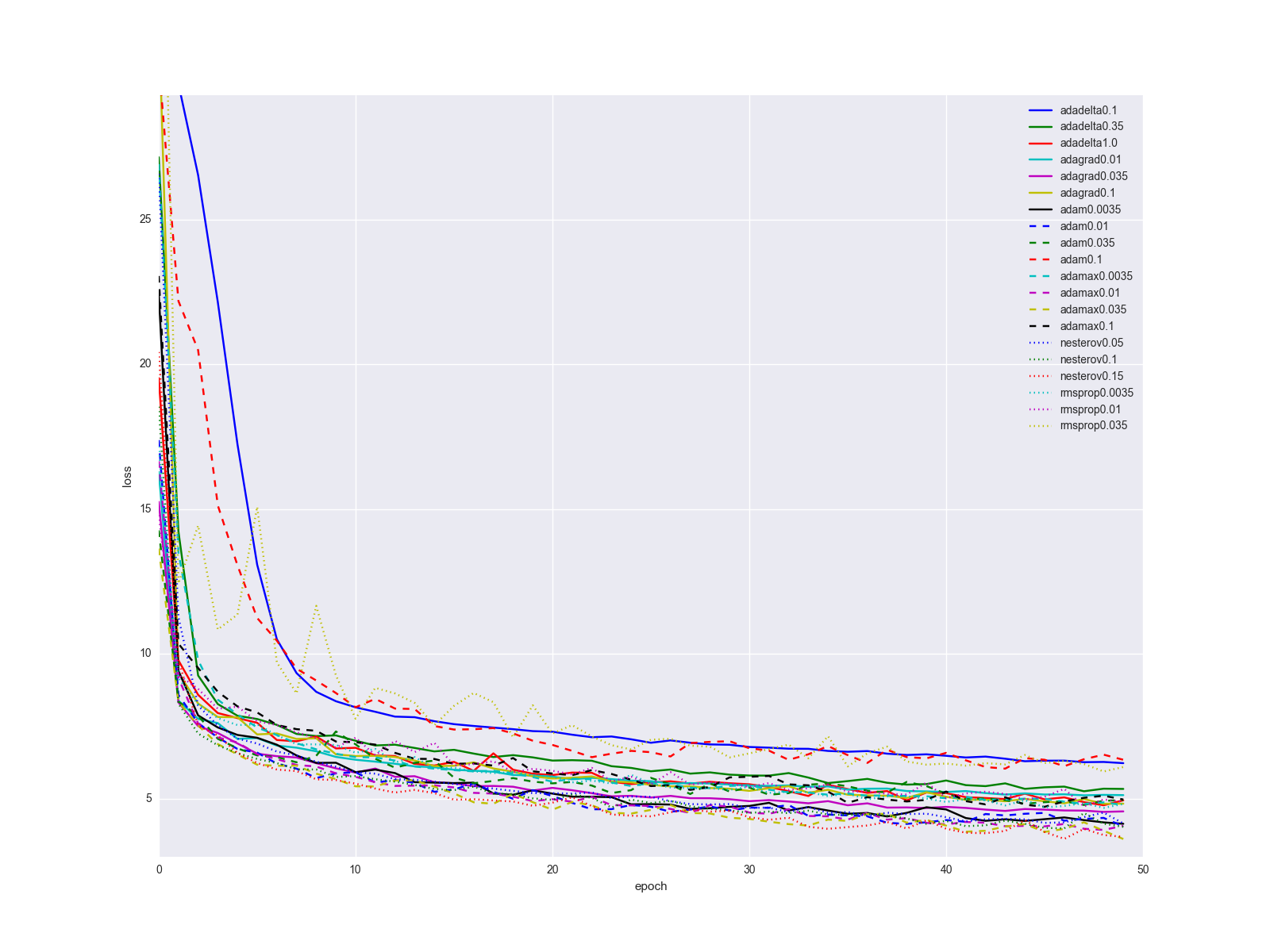
Experiments

. , . , — , , . , . , , .

$\inline \gamma$ . , , , Adam Adamax.

, -. $\inline \gamma$ SGD, . $\inline \gamma$ , , «». : , .

: , . $\inline \gamma$ , , , , .

, .

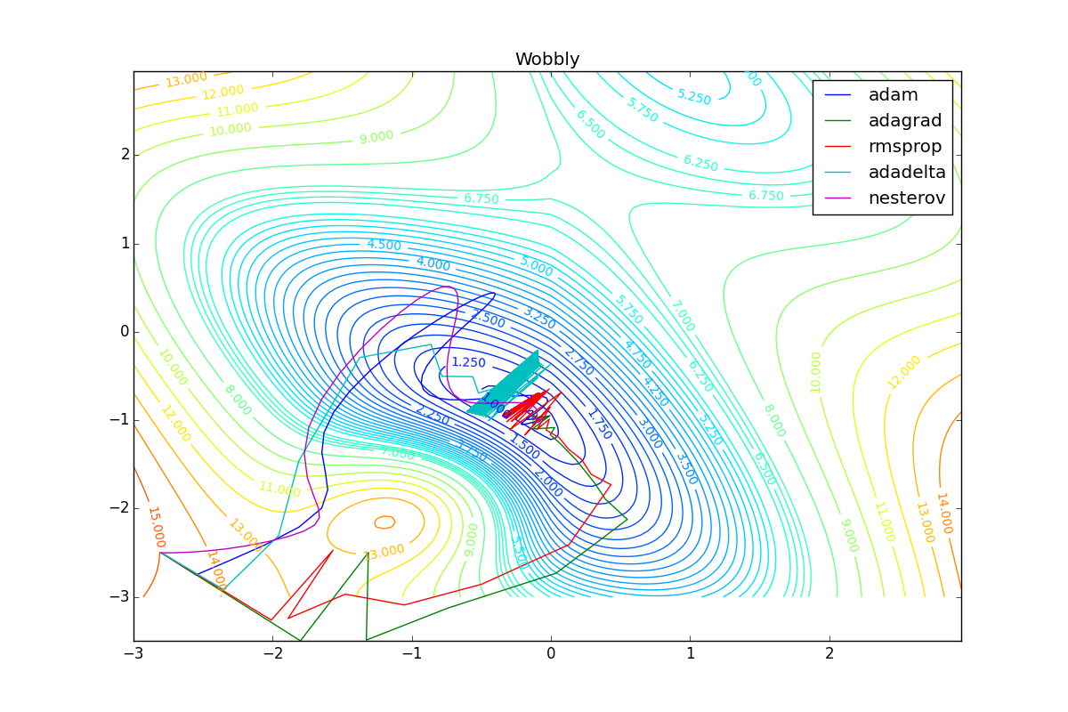
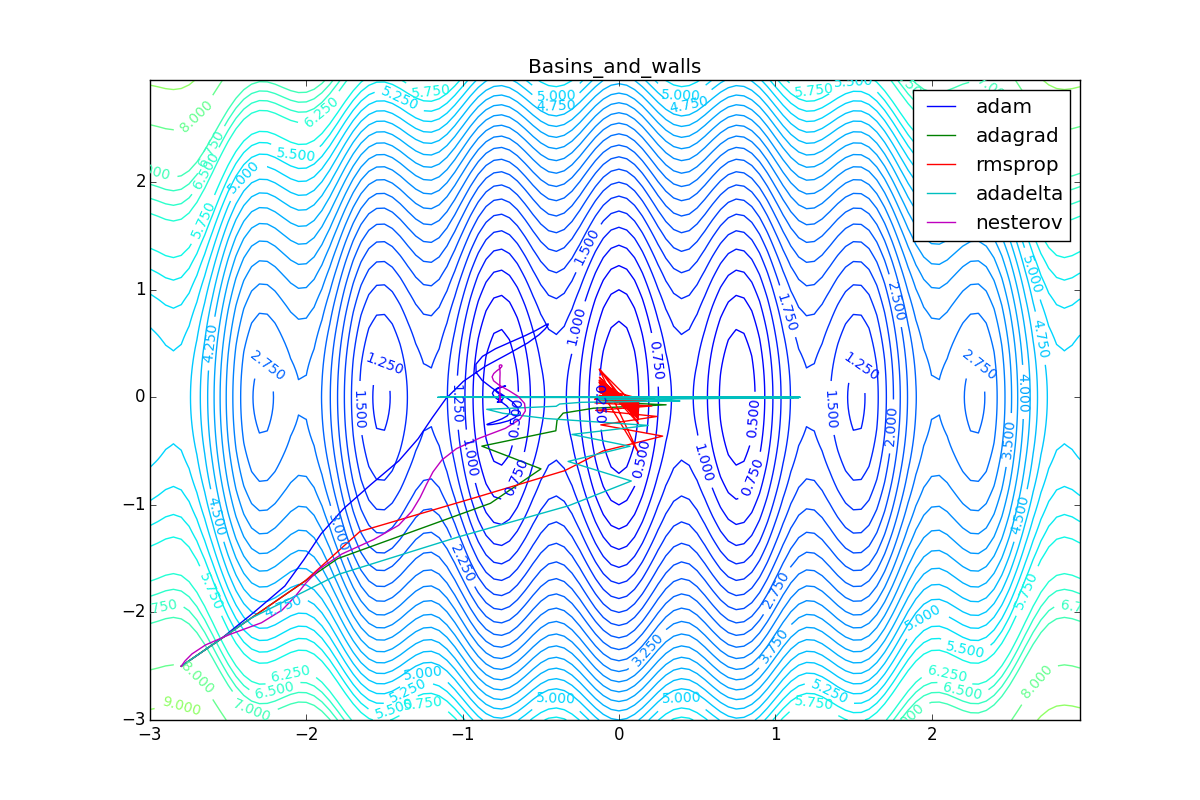
, ( ). , Adam RMSProp . ( ) (14) (23) . :

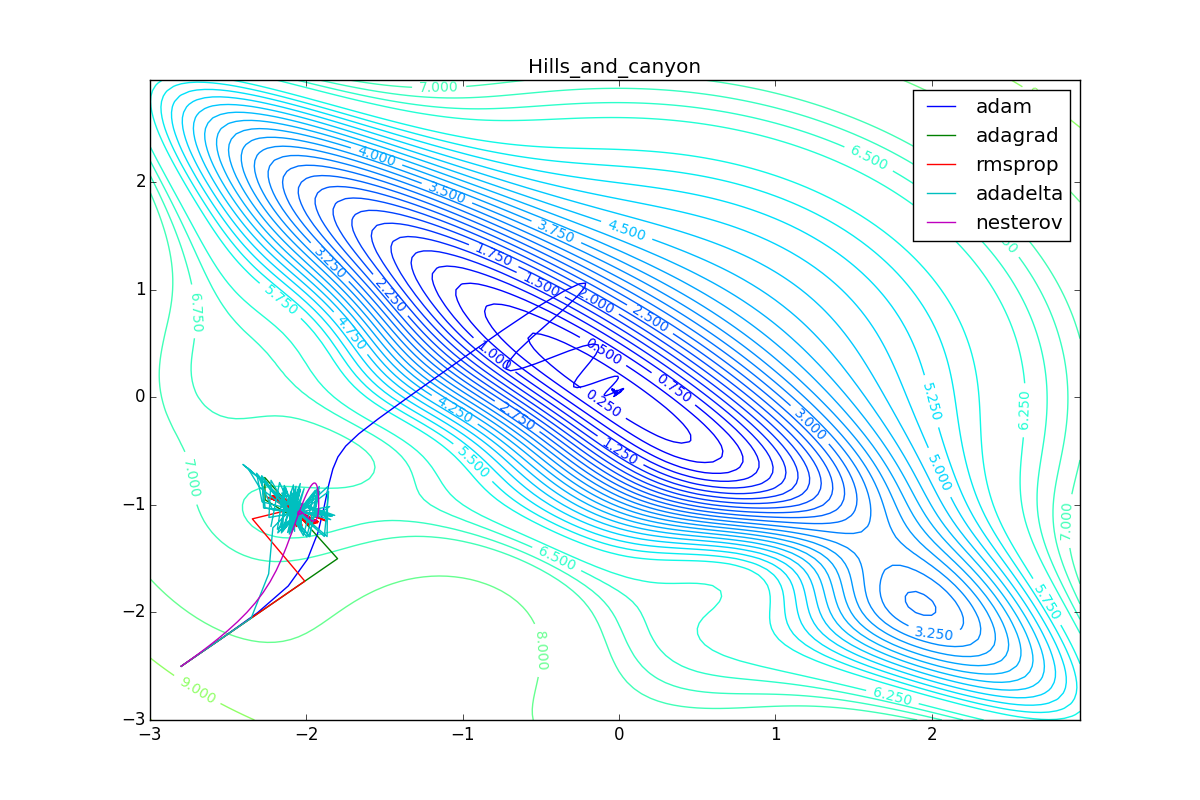
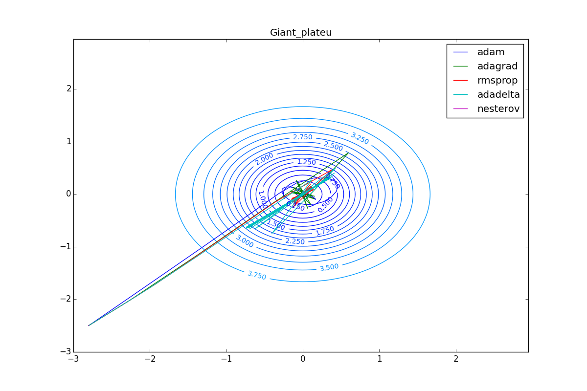
Adam, . , , RMSProp . , $\inline \gamma$ , , , - . RMSProp «». (14) — . , , ( $\inline \eta$ , ) $\inline \epsilon$ ( , ). Adagrad , , . , , , -, .

, , , , :

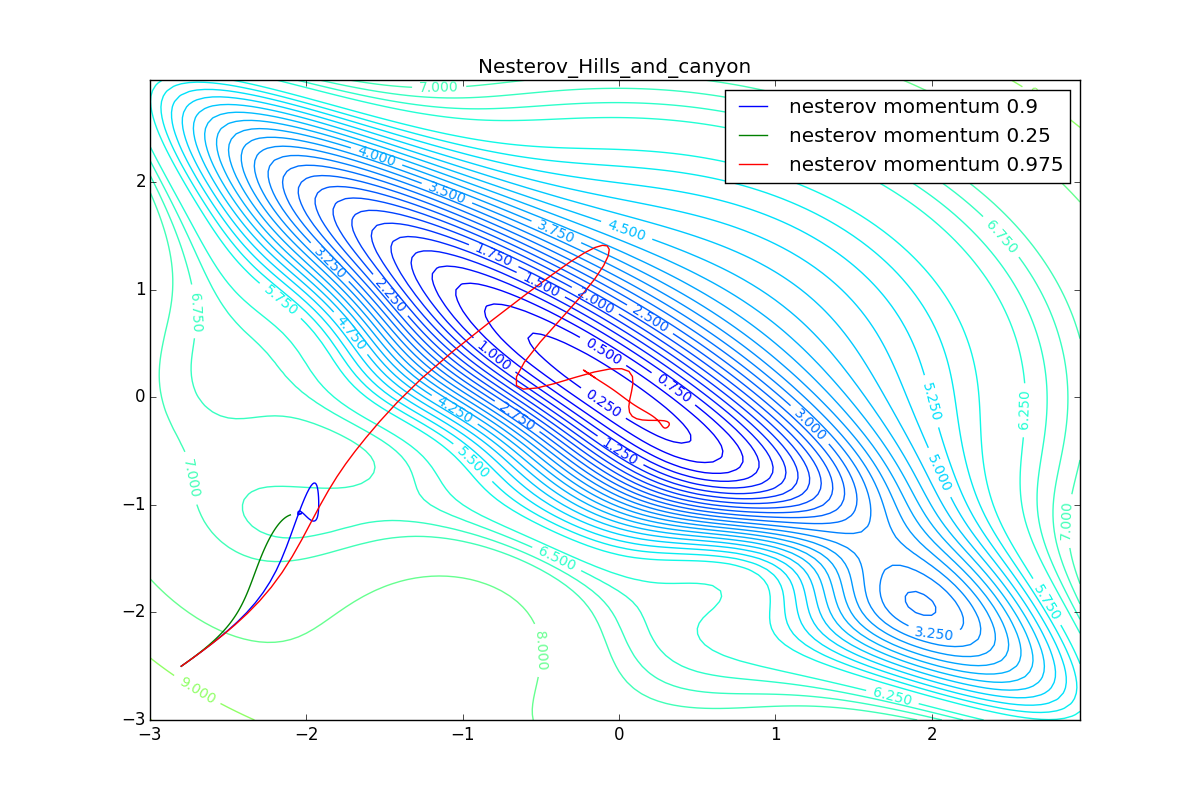
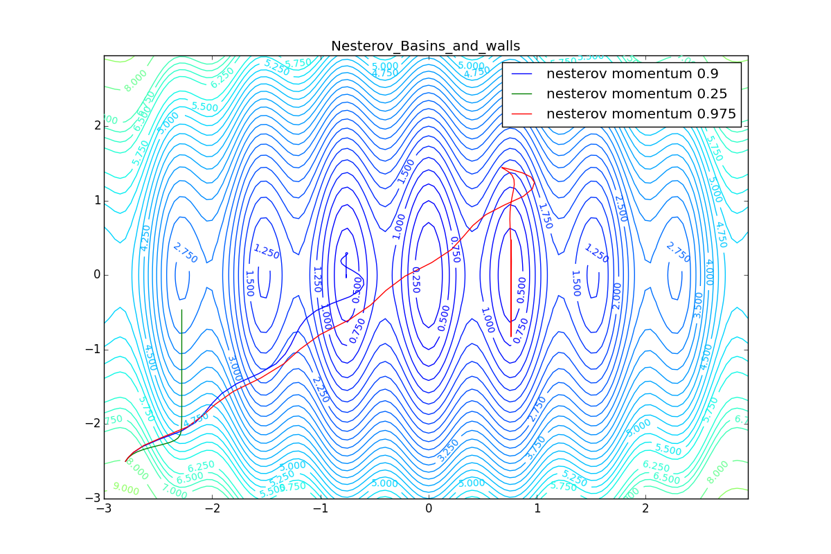
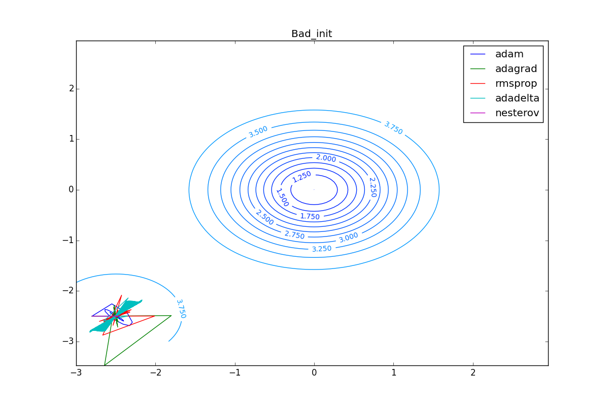
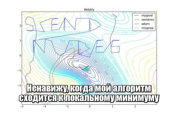
Conclusion

, . , , , .

, : . SGD - , , , - :

… . « » Adam, . - , . , . - learning rate. , - .

, ( python > 3.4, numpy matplotlib):

Code

from matplotlib import pyplot as plt import numpy as np from math import ceil, floor def linear_interpolation(X, idx): idx_min = floor(idx) idx_max = ceil(idx) if idx_min == idx_max or idx_max >= len(X): return X[idx_min] elif idx_min < 0: return X[idx_max] else: return X[idx_min] + (idx - idx_min)*X[idx_max] def EDM(X, gamma, lr=0.25): Y = [] v = 0 for x in X: v = gamma*v + lr*x Y.append(v) return np.asarray(Y) def NM(X, gamma, lr=0.25): Y = [] v = 0 for i in range(len(X)): v = gamma*v + lr*(linear_interpolation(X, i+gamma*v) if i+gamma*v < len(X) else 0) Y.append(v) return np.asarray(Y) def SmoothedNM(X, gamma, lr=0.25): Y = [] v = 0 for i in range(len(X)): lookahead4 = linear_interpolation(X, i+gamma*v/4) if i+gamma*v/4 < len(X) else 0 lookahead3 = linear_interpolation(X, i+gamma*v/2) if i+gamma*v/2 < len(X) else 0 lookahead2 = linear_interpolation(X, i+gamma*v*3/4) if i+gamma*v*3/4 < len(X) else 0 lookahead1 = linear_interpolation(X, i+gamma*v) if i+gamma*v < len(X) else 0 v = gamma*v + lr*(lookahead4 + lookahead3 + lookahead2 + lookahead1)/4 Y.append(v) return np.asarray(Y) def Adagrad(X, eps, lr=2.5): Y = [] G = 0 for x in X: G += x*x v = lr/np.sqrt(G + eps)*x Y.append(v) return np.asarray(Y) def RMSProp(X, gamma, lr=0.25, eps=0.00001): Y = [] EG = 0 for x in X: EG = gamma*EG + (1-gamma)*x*x v = lr/np.sqrt(EG + eps)*x Y.append(v) return np.asarray(Y) def Adadelta(X, gamma, lr=50.0, eps=0.001): Y = [] EG = 0 EDTheta = lr for x in X: EG = gamma*EG + (1-gamma)*x*x v = np.sqrt(EDTheta + eps)/np.sqrt(EG + eps)*x Y.append(v) EDTheta = gamma*EDTheta + (1-gamma)*v*v return np.asarray(Y) def AdadeltaZeroStart(X, gamma, eps=0.001): return Adadelta(X, gamma, lr=0.0, eps=eps) def AdadeltaBigStart(X, gamma, eps=0.001): return Adadelta(X, gamma, lr=50.0, eps=eps) def Adam(X, beta1, beta2=0.999, lr=0.25, eps=0.0000001): Y = [] m = 0 v = 0 for i, x in enumerate(X): m = beta1*m + (1-beta1)*x v = beta2*v + (1-beta2)*x*x m_hat = m/(1- pow(beta1, i+1) ) v_hat = v/(1- pow(beta2, i+1) ) dthetha = lr/np.sqrt(v_hat + eps)*m_hat Y.append(dthetha) return np.asarray(Y) np.random.seed(413) X = np.arange(0, 300) D_Thetha_spikes = np.asarray( [int(x%60 == 0) for x in X]) D_Thetha_rectangles = np.asarray( [2*int(x%40 < 20) - 1 for x in X]) D_Thetha_noisy_sin = np.asarray( [np.sin(x/20) + np.random.random() - 0.5 for x in X]) D_Thetha_very_noisy_sin = np.asarray( [np.sin(x/20)/5 + np.random.random() - 0.5 for x in X]) D_Thetha_uneven_sawtooth = np.asarray( [ x%20/(15*int(x > 80) + 5) for x in X]) D_Thetha_saturation = np.asarray( [ int(x % 80 < 40) for x in X]) for method_label, method, parameter_step in [ ("GRAD_Simple_Momentum", EDM, [0.25, 0.9, 0.975]), ("GRAD_Nesterov", NM, [0.25, 0.9, 0.975]), ("GRAD_Smoothed_Nesterov", SmoothedNM, [0.25, 0.9, 0.975]), ("GRAD_Adagrad", Adagrad, [0.0000001, 0.1, 10.0]), ("GRAD_RMSProp", RMSProp, [0.25, 0.9, 0.975]), ("GRAD_AdadeltaZeroStart", AdadeltaZeroStart, [0.25, 0.9, 0.975]), ("GRAD_AdadeltaBigStart", AdadeltaBigStart, [0.25, 0.9, 0.975]), ("GRAD_Adam", Adam, [0.25, 0.9, 0.975]), ]: for label, D_Thetha in [("spikes", D_Thetha_spikes), ("rectangles", D_Thetha_rectangles), ("noisy sin", D_Thetha_noisy_sin), ("very noisy sin", D_Thetha_very_noisy_sin), ("uneven sawtooth", D_Thetha_uneven_sawtooth), ("saturation", D_Thetha_saturation), ]: fig = plt.figure(figsize=[16.0, 9.0]) ax = fig.add_subplot(111) ax.plot(X, D_Thetha, label="gradient") for gamma in parameter_step: Y = method(D_Thetha, gamma) ax.plot(X, Y, label="param="+str(gamma)) ax.spines['bottom'].set_position('zero') full_name = method_label + "_" + label plt.xticks(np.arange(0, 300, 20)) plt.grid(True) plt.title(full_name) plt.xlabel('epoch') plt.ylabel('value') plt.legend() # plt.show(block=True) #Uncoomment and comment next line if you just want to watch plt.savefig(full_name) plt.close(fig)

If you want to experiment with the parameters of the algorithms and your own functions, use this to create your own animation of the trajectory of the minimizer (you also need theano / lasagne):

More code

 import numpy as np import matplotlib matplotlib.use("Agg") import matplotlib.pyplot as plt import matplotlib.animation as animation import theano import theano.tensor as T from lasagne.updates import nesterov_momentum, rmsprop, adadelta, adagrad, adam #For reproducibility. Comment it out for randomness np.random.seed(413) #Uncoomment and comment next line if you want to try random init # clean_random_weights = scipy.random.standard_normal((2, 1)) clean_random_weights = np.asarray([[-2.8], [-2.5]]) W = theano.shared(clean_random_weights) Wprobe = T.matrix('weights') levels = [x/4.0 for x in range(-8, 2*12, 1)] + [6.25, 6.5, 6.75, 7] + \ list(range(8, 20, 1)) levels = np.asarray(levels) O_simple_quad = (W**2).sum() O_wobbly = (W**2).sum()/3 + T.abs_(W[0][0])*T.sqrt(T.abs_(W[0][0]) + 0.1) + 3*T.sin(W.sum()) + 3.0 + 8*T.exp(-2*((W[0][0] + 1)**2+(W[1][0] + 2)**2)) O_basins_and_walls = (W**2).sum()/2 + T.sin(W[0][0]*4)**2 O_ripple = (W**2).sum()/3 + (T.sin(W[0][0]*20)**2 + T.sin(W[1][0]*20)**2)/15 O_giant_plateu = 4*(1-T.exp(-((W[0][0])**2+(W[1][0])**2))) O_hills_and_canyon = (W**2).sum()/3 + \ 3*T.exp(-((W[0][0] + 1)**2+(W[1][0] + 2)**2)) + \ T.exp(-1.5*(2*(W[0][0] + 2)**2+(W[1][0] -0.5)**2)) + \ 3*T.exp(-1.5*((W[0][0] -1)**2+2*(W[1][0] + 1.5)**2)) + \ 1.5*T.exp(-((W[0][0] + 1.5)**2+3*(W[1][0] + 0.5)**2)) + \ 4*(1 - T.exp(-((W[0][0] + W[1][0])**2))) O_two_minimums = 4-0.5*T.exp(-((W[0][0] + 2.5)**2+(W[1][0] + 2.5)**2))-3*T.exp(-((W[0][0])**2+(W[1][0])**2)) nesterov_testsuit = [ (nesterov_momentum, "nesterov momentum 0.25", {"learning_rate": 0.01, "momentum": 0.25}), (nesterov_momentum, "nesterov momentum 0.9", {"learning_rate": 0.01, "momentum": 0.9}), (nesterov_momentum, "nesterov momentum 0.975", {"learning_rate": 0.01, "momentum": 0.975}) ] cross_method_testsuit = [ (nesterov_momentum, "nesterov", {"learning_rate": 0.01}), (rmsprop, "rmsprop", {"learning_rate": 0.25}), (adadelta, "adadelta", {"learning_rate": 100.0}), (adagrad, "adagrad", {"learning_rate": 1.0}), (adam, "adam", {"learning_rate": 0.25}) ] for O, plot_label in [ (O_wobbly, "Wobbly"), (O_basins_and_walls, "Basins_and_walls"), (O_giant_plateu, "Giant_plateu"), (O_hills_and_canyon, "Hills_and_canyon"), (O_two_minimums, "Bad_init") ]: result_probe = theano.function([Wprobe], O, givens=[(W, Wprobe)]) history = {} for method, history_mark, kwargs_to_method in cross_method_testsuit: W.set_value(clean_random_weights) history[history_mark] = [W.eval().flatten()] updates = method(O, [W], **kwargs_to_method) train_fnc = theano.function(inputs=[], outputs=O, updates=updates) for i in range(125): result_val = train_fnc() print("Iteration " + str(i) + " result: "+ str(result_val)) history[history_mark].append(W.eval().flatten()) print("-------- DONE {}-------".format(history_mark)) delta = 0.05 mesh = np.arange(-3.0, 3.0, delta) X, Y = np.meshgrid(mesh, mesh) Z = [] for y in mesh: z = [] for x in mesh: z.append(result_probe([[x], [y]])) Z.append(z) Z = np.asarray(Z) print("-------- BUILT MESH -------") fig, ax = plt.subplots(figsize=[12.0, 8.0]) CS = ax.contour(X, Y, Z, levels=levels) plt.clabel(CS, inline=1, fontsize=10) plt.title(plot_label) nphistory = [] for key in history: nphistory.append( [np.asarray([h[0] for h in history[key]]), np.asarray([h[1] for h in history[key]]), key] ) lines = [] for nph in nphistory: lines += ax.plot(nph[0], nph[1], label=nph[2]) leg = plt.legend() plt.savefig(plot_label + '_final.png') def animate(i): for line, hist in zip(lines, nphistory): line.set_xdata(hist[0][:i]) line.set_ydata(hist[1][:i]) return lines def init(): for line, hist in zip(lines, nphistory): line.set_ydata(np.ma.array(hist[0], mask=True)) return lines ani = animation.FuncAnimation(fig, animate, np.arange(1, 120), init_func=init, interval=100, repeat_delay=0, blit=True, repeat=True) print("-------- WRITING ANIMATION -------") # plt.show(block=True) #Uncoomment and comment next line if you just want to watch ani.save(plot_label + '.mp4', writer='ffmpeg_file', fps=5) print("-------- DONE {} -------".format(plot_label))

→ PDF version of the article

Thanks to Roman Parpalak for the tool thanks to which working with formulas on the habr is not so painful. You can see the article that I took for the basis of my article - there is a lot of useful information that I omitted in order to better focus on optimization algorithms. To further delve into the neural networks, I recommend this book.

Have a good New Year's Eve weekend, Habr!

Source: https://habr.com/ru/post/318970/

All Articles