Classifiers: analysis of site visitors activity

1. Introduction

This article describes some aspects of the practical application of classifiers in the systems for analyzing the activity of site visitors. Code examples for machine learning tasks are shown, which are actively used both for global analysis of statistics on the Internet and for local tasks of behavioral factor classification on large portals.

2. Some methods of probability theory

The main problem lies in the fact that with stochastic processes (activity of site visitors) it is impossible to identify in advance the value of a random variable. However, we can estimate the probability of each of the values. Moreover, using the methods of machine learning we can understand the reasons why a particular random variable took its value.

There are stochastic processes with a very sharply pronounced regularity, for example, the observer recorded several thousand tests. Suppose that for the entire long period of observations it was found that the random variable took only four possible values ​​with an equal distribution. It is logical to assume that the number of one of these values ​​will be about four times less than the number of all. And vice versa: by multiplying the number of values ​​from one group by four, we get an approximate number of all objects.

By analogy, it is possible to identify (using the Monte Carlo method) the approximate area of ​​complex figures, if you know the number of hits on the point, the total number of random points and the area of ​​the space in which the complex figure is inscribed. It will be intuitively felt that if you divide the number of hits in a complex figure by the total number of points, then this will be the approximate part that the figure takes in space. Moreover, it will also be the probability of hitting a point in this complex figure.

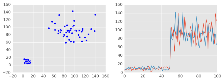
Consider a simplified example. Suppose there are four main topics on the huge news portal. Some users come to the site and watch strictly only one of the topics. The distribution between them is equal, i.e. equal probability that the topic of one of the clusters will be viewed. But the exact position of the new point is not known in advance, and it is only known that it will necessarily appear in one of these clusters (centroids are shown as large green dots):

It is impossible for a non-existent topic to be viewed (how can I see it if it is not there?), I.e. its probability is zero. Any point belongs only to this space. The probability of hitting a particular cluster is 1/4. The probability of hitting at least one of the clusters will be equal to 1 (the sum of the probabilities of all events), since the point necessarily falls into one of them. The probability that the points fall into one cluster several times in a row is equal to the product of the probabilities of these events. This can be seen experimentally and formally written as:

But for normal distribution, a slightly different prediction tactic is used. It is necessary to identify the average value. That it will be the most likely. Next, I present two visual images of an equiprobable distribution and a normal distribution.

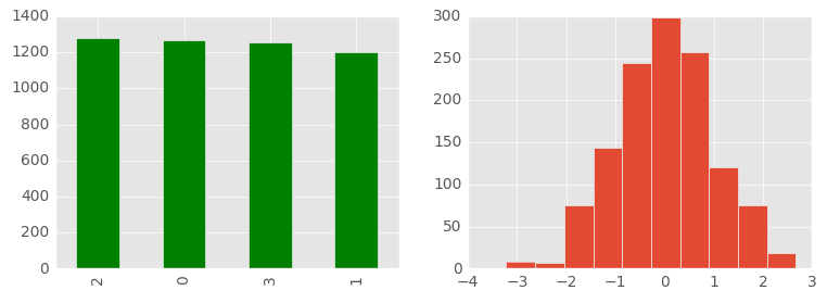
To understand the power of variation, it is necessary to identify the variance (or the square root of it, which is called the standard deviation and is denoted by the Greek letter sigma). To predict the value of a discrete random variable is a very important indicator, since most of the values ​​(if it is a normal distribution) are within sigma limits.

In other words: if in a normal distribution we expect the arithmetic average (it is equal to the expectation), and the allowable error (inaccuracy or error) is at least about one sigma, then in most cases (about 68%) we will successfully guess. Visually we will display a random variable with a different level of dispersion: at first, the dispersion is small, and then it clearly increases. For the convenience of visual perception, the expectation is also increased.

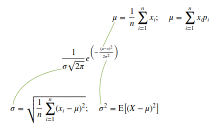
Since we are talking about discrete random variables, it is permissible to use the arithmetic mean value formula instead of the expectation formula. For the reason mentioned, you can use the formula shown at the bottom left in order not to calculate the sum of the square of the value multiplied by the probability, and then subtract the square of the expected value from the sum of these products. I present the normal distribution function and the variables necessary for it (formulas for calculating them):

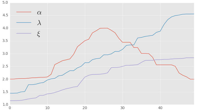
But not always everything is so predictable. Naturally, the probability of a random variable may vary. Not all processes will have Gaussian distribution or an equiprobable distribution. Very often, it is possible to record changes in probability with time, i.e. Some metrics can change their values ​​in unpredictable ways, which will obviously affect probability. An example of a change in values ​​in which two metrics grow unevenly, and one after growth returns to its original value:

Consequently, in a number of processes, the results (the appearance of a point) may not be evenly distributed. Obviously, in the following example, the cloud cannot be called evenly distributed in space. For clarity, I also cite its contours:

In the analysis of a large number of data with different distributions, machine learning will help us. Each observation will have a large feature vector. For example, in the diagnosis of ARVI often use such an indicator as body temperature. It is very easy to measure it objectively using an appropriate instrument. Obviously, if you look at the descriptive statistics of the body temperature of two groups of people (healthy and with ARVI), then it will be easy enough to understand the differences in this indicator. Of course, one metric will not be enough, as a symptom of fever may occur (or be absent) in many other diseases. Therefore, we need to objectively measure a huge list of indicators (vector of predictors). Each vector must have a label: healthy or sick. This is a general principle of data preparation for those machine learning methods that will be discussed now.

3. Preliminary study

The preliminary stage of the analysis does not always require the use of servers in the data center, therefore, it is performed on local computers. One of the most popular data analysis tools are the programming languages ​​R and Python (in combination with Jupyter, Pandas, NumPy and SciPy). They have a rich set of already implemented mathematical functions and tools for visualizing information.

At the stage of preliminary research it is necessary to collect the necessary information for classification. This is always a feature vector, i.e. numbers (usually the Double data type). At this stage, the methods of collection and actions are selected in case of impossibility to obtain a value (it is sometimes permissible to replace the missing values ​​with the arithmetic mean or median).

The metric (predictor) should be such a number that objectively reflects the essence of this part of the phenomenon. Such a metric is measurable, and the measurements themselves are reproducible (anyone with a working measuring device can repeat the experiment and get about the same indicators). It is intuitively expected that the stronger the difference between the values ​​of a metric in different groups, the easier it will be to classify. In the most ideal case, they do not intersect (the maximum of one is clearly less than the minimum of the other).

Additional checks may also be required at this stage. They are implemented using a very large number of third-party libraries and software products. Sometimes it is fun to watch the number of imported modules, especially at first glance, a different purpose (like Mystem and Selenium). It is logical that you can perform various experiments that confirm or refute the hypothesis. Subdivide and, under close monitoring, reproduce the conditions and expect changes in metrics accordingly.

If we talk about the specifics of systems for analyzing behavioral factors, the logic of their work implies that the collected data have already been cleared and validated. Ideally, the application itself should be responsible for the quality of data collection. It remains only to mark (for each vector, mark the class to which it belongs). It is possible that the application has already marked the data (for example, there is already an entry in the database, which will become a label: bought or not bought the product). Of course, this is necessary in order to further predict the probability of this event or to identify the most important predictors.

Quite often, data is stored in plain text files in CSV or libsvm format. This allows you to conveniently process them using R and Python (Pandas, NumPy). In some cases it is necessary to put them in a database. And in some cases, distributed computing may be required. On huge portals and in global statistical systems, a very large matrix is ​​obtained. This raises the question of choosing a system for storing a huge number of observations in a very wide table (there are a lot of tuples with a large number of attributes).

Most likely, it makes sense to pay attention to specialized analytical solutions that have tremendous processing speed. The use of technologies such as ClickHouse (analytical database management system) allows you to pre-analyze some important indicators and prepare the data itself. And now it's not just about high performance, but also about a number of useful functions for working with statistics, as well as additional features, such as the choice of data export format (including JSON and XML) or the answer directly in the browser after a get request ( http: // localhost: 8123 /? query = Q ), where instead of Q the following expression in SQL:

SELECT page, COUNT() AS views, uniqCombined(uuid) AS users FROM example.page_views GROUP BY page FORMAT CSVWithNames; 

The preparation and verification of data is a very serious process, they pay great attention to it. After several research requests, the selection of machine learning algorithms and a more detailed analysis of the sample with the tools mentioned earlier begin. Even at the stage of selecting the most appropriate classification algorithms, the verification of the initial data and the attempt to find new predictors continues. In any case, very many “classification wonders” are easily explained by a couple of missed or noisy predictors. In some cases, you can even create an array of classifiers and analyze the correct operation of each of them with the appropriate parameters:

 import pylab import pandas as pd import numpy as np import xgboost as xgb import matplotlib.pyplot as plt from sklearn.cluster import KMeans from mpl_toolkits.mplot3d import Axes3D from sklearn.linear_model import SGDClassifier from sklearn.neural_network import MLPClassifier from sklearn.ensemble import RandomForestClassifier from sklearn.ensemble import GradientBoostingClassifier from sklearn.linear_model import LogisticRegression from sklearn.tree import DecisionTreeClassifier from sklearn.svm import SVC from sklearn.metrics import accuracy_score from IPython.core.display import display, HTML # #   # classifiers = [ LogisticRegression(max_iter=200, penalty="l2"), SGDClassifier(loss="hinge", penalty="l2"), MLPClassifier(solver='lbfgs', alpha=1e-5, hidden_layer_sizes=(3, 4)), RandomForestClassifier(n_estimators=60, max_depth=5), GradientBoostingClassifier(n_estimators=180, learning_rate=1.0, max_depth=4), DecisionTreeClassifier(), SVC(), ] # #     # result = [] for classifier in classifiers: classifier.fit(features, classes) report = accuracy_score(testClasses, classifier.predict(testFeatures)) result.append({'class' : classifier.__class__.__name__, 'accuracy' : report}) display(HTML('<h2>Result</h2>')) display(pd.DataFrame(result)) # #     # model = xgb.XGBClassifier() model.fit(features, classes) pylab.rcParams['figure.figsize'] = 3, 3 plt.style.use('ggplot') pd.Series(model.feature_importances_).plot(kind='bar') plt.title('Feature Importances') plt.show()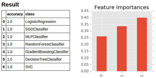 

As you can see, the main classification algorithms are already implemented in popular libraries, which makes it very easy and quick to use them with just a few lines of code. In addition, it is very useful for some models to look at the diagram of the significance of predictors using suitable classifiers (such as: RandomForestClassifier, GradientBoostingClassifier, XGBClassifier). It is very convenient to perform other types of data analysis and visualization, for example, cluster analysis:

 import pylab import pandas as pd import numpy as np import matplotlib.pyplot as plt from sklearn.cluster import KMeans from mpl_toolkits.mplot3d import Axes3D centroids = KMeans(n_clusters=4, random_state=0).fit(features).cluster_centers_ ax = Axes3D(pylab.figure()) ax.scatter(features[:, 0], features[:, 1], features[:, 2], c='blue', marker='p', s=8) ax.scatter(centroids[:, 0], centroids[:, 1], centroids[:, 2], c='g', marker='o', s=80) plt.show() 

4. Creating a finished model

Once the appropriate algorithm with the necessary parameters has been selected on the local system, the preparation of distributed computations begins, the task of which is to predict the event class in advance. This may be not just a binary classification (an event will happen or not), but a multi-class classification. For such tasks, distributed computing often uses Apache Spark (examples are shown on Scala for version 2.0.2). Of course, the first test runs also require a very thorough check of the chosen solution on the new data:

 import org.apache.spark.ml.classification.MultilayerPerceptronClassifier import org.apache.spark.ml.evaluation.MulticlassClassificationEvaluator val train = spark.read.format("libsvm").load(file) val test = spark.read.format("libsvm").load(fileTest) val trainer = new MultilayerPerceptronClassifier().setLayers(Array[Int](3, 5, 4, 4)).setBlockSize(128).setSeed(1234L).setMaxIter(100) val result = trainer.fit(train).transform(test) val predictionAndLabels = result.select("prediction", "label") val evaluator = new MulticlassClassificationEvaluator() evaluator.setMetricName("accuracy").evaluate(predictionAndLabels) 

At the end of the verification and adjustment process, the final version of the machine learning algorithm begins its work. It marks the huge data arrays, and the results are displayed in a user-friendly interface. A separate application is responsible for rendering (often this is a web application or part of a portal). As a rule, the application does not know anything about the analysis system, and is associated with it only by importing it into a database or through an API. In my personal experience, a well-known technology stack (PHP7, Yii 2, Laravel, MySQL, Redis, Memcached, RabbitMQ) for the backend and a set of libraries for visual presentation (for example, Chart.js and many others) are usually used for a separate display application.

Thus, we took a look at the basic steps of creating a system for analyzing behavioral factors. Systems for classifying other data sets work in a similar way. The most basic steps can be called the collection of correct metrics in a suitable format (as they say, “expand into a vector”) and the choice of a suitable algorithm with the necessary parameters. Of course, it is crucial to check the correctness of the classifier.

Taking this opportunity (taking into account today's date), I congratulate dear readers in advance on the coming new year and absolutely sincerely wish you happiness and success in all spheres of life.