Poisson distribution and football betting

If we combine the statistics of sports competitions with the Poisson distribution, then we can calculate the probable number of balls that will be scored during a football game. On this basis, it is possible to understand where the betting rates are taken from, and also learn how to calculate them yourself using R.
At the end of the XIX century. Russian economist and statistician of Polish origin, Vladislav Bortkiewicz, after analyzing the data in 14 corps of the Prussian army for 20 years, came up with a way to predict the deaths of soldiers from hitting a horse. For this, he was one of the first to use the Poisson distribution in practice. The results of his calculations are shown in the table.
| Horse mortality | According to the Poisson formula | Observations |
|---|---|---|
| 0 | 108.67 | 109 |
| one | 66.29 | 65 |
| 2 | 20.22 | 22 |
| 3 | 4.11 | 3 |
| four | 0.63 | one |
| five | 0.08 | 0 |
| 6 | 0.01 | 0 |
As we see, probability-theoretic calculations are perfectly combined with real data. Can I use this method in sports betting to have fun and earn money?
Poisson formula
In the textbook on probability theory B. V. Gnedenko, this definition of the Poisson theorem is given.
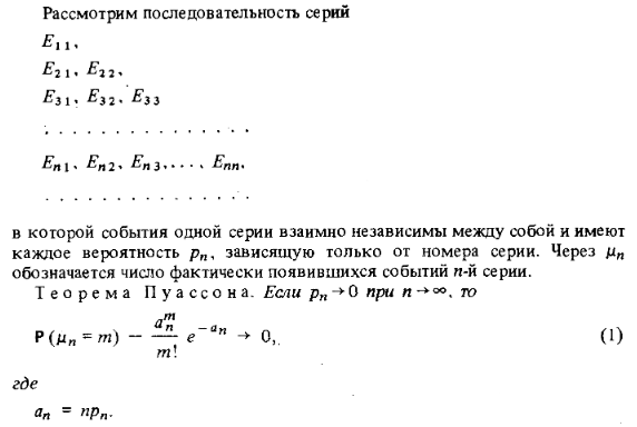
If we speak in simple language, then on the basis of this formula, it is possible to calculate the probability distribution for events that:
- occur per unit of time or per unit area;
- discrete, they can be numbered;
- independent of each other;
- do not have an upper limit, at least - theoretical;
We can cite a lot of examples from everyday life: the number of people affected by lightning, traffic accidents, the number of advertising calls and messages, the number of elevator failures per year, the highlights in the Easter cake, etc. For us, examples from sports are of interest.
Football statistics
It turns out that the number of goals scored in a football match fits very well into the Poisson distribution. So, in the diagram on the left, we see the number of goals scored by each team in each of the 380 matches of the 2008–09 Spanish Championship. The diagram on the right is calculated theoretical data of the model.
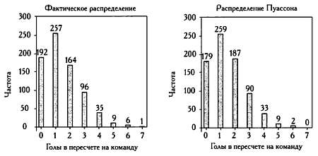
The diagrams are very similar, therefore there is reason to believe that the Poisson model can explain the ratio of the goals scored by the team during the match.
Now a little about sports betting. Those who drop in the bookmakers can see them on the scoreboard. This is how some of the bets on the English Premier League teams play this Monday.
| England - Premier League | one | x | 2 |
|---|---|---|---|
| Manchester United - Sunderland | 1.25 | 6.80 | 15.00 |
| Chelsea - Bournemouth | 1.39 | 5.10 | 10.50 |
| Hull - Manchester City | 10.50 | 5.80 | 1.35 |
1 - first team win
x - draw
2 - the victory of the other team.
It is enough to glance at the standings and it will be clear why the stakes and the possible win are so high if Sunderland wins over Manchester United. For each ruble in this case, you can earn 15 rubles, in the case of the victory of the Manchester United team, the gain will be only 1.25 rubles.
Let us now try to calculate the bets on the game Manchester United against Manchester City, which is to be held on February 26, 2017 . Despite the fact that the two clubs have similar names, MS plays in their field, and MJ - at a party.
Before using the Poisson formula, it is necessary to calculate the value of µ , and for this you need to get the average number of players scored and missed balls relative to the average for all teams.
µ MU - Estimated number of goals scored for Manchester United
µ MC - Expected number of goals scored for Manchester City
Then
- µ MU = MJ attack ✕ MC defense ✕ average number of goals scored at away matches.
- µ MC = attack MC ✕ defense MJ ✕ average number of goals scored in his field.
For the entire season 2015/2016 there were 380 football games in which teams scored 567 goals at home (1.49 per game), and away - 459 (1.20 per game).
(5:563)$ echo 'scale=5;567/380;459/380' | bc -q 1.49210 1.20789 Further, we consider the attack rates of the Ministry of Justice, the attacks of the Movement of Defense, the defense of the Ministry of Justice and the Defense of the MC.
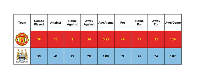
At away matches Manchester United scored an average of 1.15 goals per game, and missed - 1.36.
(5:552)$ echo 'scale=5;22/19;26/19' | bc -q 1.15789 1.36842 At home, Manchester City scored an average of 2.47 goals per game, and missed - 1.10.
(5:553)$ echo 'scale=5;47/19;21/19' | bc -q 2.47368 1.10526 Now we are weighing the same values relative to the total average values. The relative average of MJ attacks in a foreign field is 0.958, and the relative average of the MF defense in its field is 0.915.
(5:554)$ echo 'scale=5;22/19/1.20789;21/19/1.20789' | bc -q .95860 .91503 The relative average defense of the Ministry of Justice in a foreign field is 0.917, and the relative average of the MC attacks in their field is 1.657.
(5:555)$ echo 'scale=5;26/19/1.49210;47/19/1.49210' | bc -q .91711 1.65785 Finally, multiplying all intermediate averages, we find µ .
µ MU = 1.06
µ MC = 2.27
(5:556)$ echo 'scale=5;.95860*.91503*1.20789;1.65785*.91711*1.49210' |bc -q 1.05948 2.26863 Poisson Goals
Now we can calculate the probabilities for different outcomes of this meeting. In R this is done very simply, but you can cut corners and use the statistical online calculator .
> dpois(x=(0:5), lambda=2.26863) [1] 0.10345381 0.23469843 0.26622195 0.20131970 0.11417998 0.05180642 > dpois(x=(0:5), lambda=1.05948) [1] 0.346636014 0.367253924 0.194549094 0.068706958 0.018198412 0.003856171 So, the probabilities are distributed as follows.
| Goals | 0 | one | 2 | 3 | four | five |
|---|---|---|---|---|---|---|
| MJ | 34.663% | 36.725% | 19.454% | 6.870% | 1.819% | 0.385% |
| MS | 10.345% | 23.469% | 26.622% | 20.131% | 11.417% | 5.180% |
The probability that Manchester United does not score a single goal is 34.663%, the same is for Manchester City - 10.345%, the probability of a zero outcome of the meeting is equal to their product and is 3.586%. Matrix of all results from 0: 0 to 5: 5.
> a=dpois(x=(0:5), lambda=1.05948) > b=dpois(x=(0:5), lambda=2.26863) > A=a%*%t(b) > A [,1] [,2] [,3] [,4] [,5] [,6] [1,] 0.0358608180 0.0813549276 0.092282115 0.0697846579 0.0395788921 0.0179579724 [2,] 0.0379938195 0.0861939186 0.097771055 0.0739354494 0.0419330446 0.0190261126 [3,] 0.0201268459 0.0456603665 0.051793239 0.0391665649 0.0222136111 0.0100788929 [4,] 0.0071079969 0.0161254150 0.018291300 0.0138320641 0.0078449589 0.0035594618 [5,] 0.0018826951 0.0042711387 0.004844817 0.0036636988 0.0020778943 0.0009427947 [6,] 0.0003989356 0.0009050372 0.001026597 0.0007763231 0.0004402975 0.0001997744 Now let's try to calculate the probability of victory for each side, the likelihood of a drawn outcome, and finally we will determine the stakes. Let's start with a draw. Multiply the event vectors for MJ and MS, and assume the sum of the diagonal matrix. Bet 1 to 5.264 .
> sum(diag(A)) [1] 0.1899577 > 1/sum(diag(A)) [1] 5.26433 The chances of the MC winning are equal to the sum of all possible 1: 0, 2: 0, ... 5: 0, 2: 1, 3: 1, ..., etc., up to 5: 4. The bet is 1.619 .
sum(A[1,2:6])+sum(A[2,3:6])+sum(A[3,4:6])+sum(A[4,5:6])+A[5,6] [1] 0.6174305 1/(sum(A[1,2:6])+sum(A[2,3:6])+sum(A[3,4:6])+sum(A[4,5:6])+A[5,6]) 1.619615 The chances of winning a MJ are smaller, respectively, there will be more bet and a cash prize - 1 to 5.191 .
> 1 - (sum(A[1,2:6])+sum(A[2,3:6])+sum(A[3,4:6])+sum(A[4,5:6])+A[5,6] + sum(diag(A))) [1] 0.1926118 > 1/(1 - (sum(A[1,2:6])+sum(A[2,3:6])+sum(A[3,4:6])+sum(A[4,5:6])+A[5,6] + sum(diag(A)))) [1] 5.19179 Bets are made!
| Game bets | one | x | 2 |
|---|---|---|---|
| Manchester City - Manchester United | 1.620 | 5.264 | 5.192 |
Of course, the Poisson model is quite simple and does not take into account many factors and circumstances: a new player, a new coach, match status, club circumstances, etc. Nevertheless, Elihu Feustel manages to earn millions by betting using mathematical algorithms.
Used materials
')
Source: https://habr.com/ru/post/318150/
All Articles