Looking for familiar faces
In the article I want to acquaint the reader with the task of identification: walk from the basic definitions to the implementation of one of the recent articles in this area. The result should be an application that can search for the same people in the photos and, most importantly, an understanding of how it works.
The Bourne Identification (and not only the Bourne)

The task of identification is similar to the task of classification and historically arose from it, when instead of determining the class of an object, it became necessary to be able to determine whether an object has the required property or not. In the identification task, the training set is a set of objects

For example, if you want to separate the faces of people from the faces of monkeys, then this is a classification task - there are two classes, for each object you can specify a class and make a representative sample of both classes. If it is required to determine to which person the face image belongs and these people are a finite fixed set, then this is also a classification task.
Now imagine that you are developing an application that should determine a person from a photo of his face, and many people remembered in the database are constantly changing and, naturally, during use, the application will see people who were not in the training set - a real task, which Today’s world is no surprise. However, it is no longer limited to the task of classification. How to solve it?
To be able to recognize a person, you must see him at least once. Or rather, to have at least one of his photos or to remember it in the form of some image. Then, when we are shown a new, previously unknown photograph, we will compare it with all the memorized images and will be able to give an answer: we have already seen this person and can identify him or this person has never met us before and we can only remember him. Thus the task stated above is reduced to the following: having two photos
')
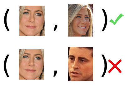
Here is the definition of the task of identification: according to the training sample (in the example: many pairs of faces
We will set the last problem from the example in a slightly more formal and heroic way of solving it, calling arxiv.org , Python, and Keras for help. Face photos - matrix of
Superiority bourne
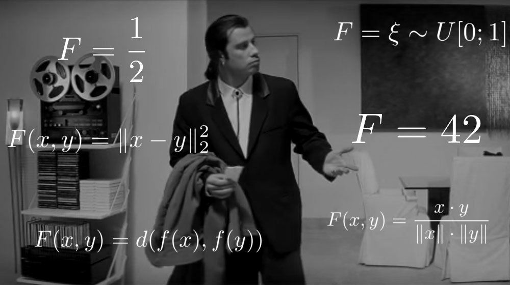
What is most important in solving the problems of machine learning? Do you think the ability to search for an answer? No, the main thing is the ability to verify this answer. Function
Let's introduce the concept of target attempts and imposter tests. First we name the object
Now let's take our constructed function.
So she looks for

Agree, the sense of such an identifier is a little - in half of the cases it will guess the answer, and in half it will be wrong.
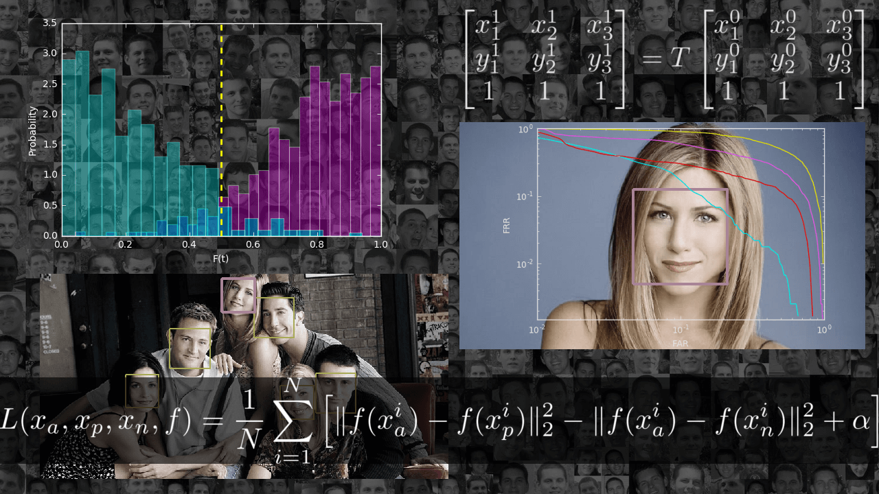
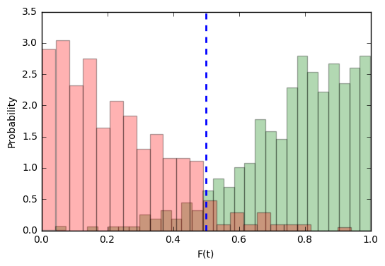
This distribution suits us better:
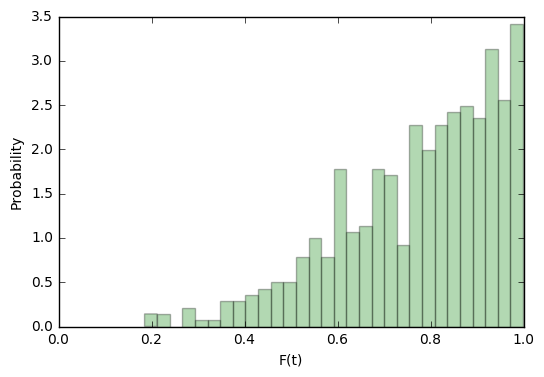
For target attempts, such a function will be more confident in their correctness than not.
But consideration of the distribution of the target without the distribution of imposters is meaningless. Let's do the same operation for them: build the distribution density

It becomes clear that for imposter attempts, our function will in most cases be inclined to the correct answer. But these are still only visual observations; they do not give us any objective assessment.
Suppose our system is fed a couple of images at the entrance. She can calculate for them the probability that this is a target . But it requires an unequivocal answer from her: whether it is the same person or not, whether to let him on a secret object or not. Let's set some threshold
In how many cases will our system be wrong with target attempts? Easy to count:
- FRR (False Rejection Rate) - the proportion of incorrectly rejected target attempts.
- FAR (False Acceptance Rate) - the proportion of incorrectly taken imposter- attempts.
Let's now take some step.
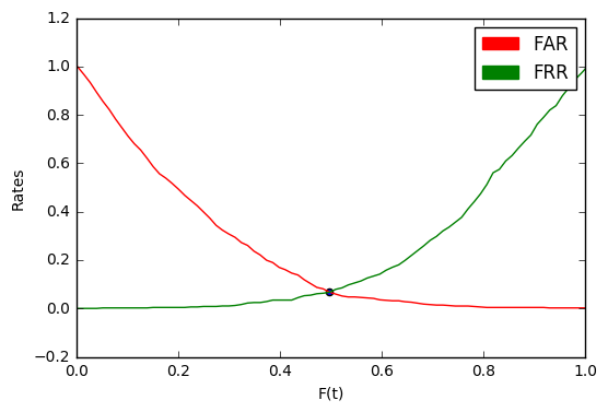
Now, for any chosen distance, we can say what proportion of target attempts will deviate and what proportion of imposter attempts will be taken. Conversely, you can choose
Pay attention to the point of intersection of the graphs. The value in it is called EER (Equal Error Rate).
If we choose
In the example above, EER = 0.067. This means that on average 6.7% of all target attempts will deviate and 6.7% of all imposter attempts will be accepted.
Another important concept is the DET curve - the dependence of FAR on FRR on a logarithmic scale. By its form it is easy to judge the quality of the system as a whole, to evaluate what value of one criterion can be obtained with a fixed second, and, most importantly, compare systems.

ERR here is the intersection of a DET curve with a straight line.
A naive implementation in Python (you can be more optimal if you consider that FAR and FRR change only at points from
import numpy as np def calc_metrics(targets_scores, imposter_scores): min_score = np.minimum(np.min(targets_scores), np.min(imposter_scores)) max_score = np.maximum(np.max(targets_scores), np.max(imposter_scores)) n_tars = len(targets_scores) n_imps = len(imposter_scores) N = 100 fars = np.zeros((N,)) frrs = np.zeros((N,)) dists = np.zeros((N,)) mink = float('inf') eer = 0 for i, dist in enumerate(np.linspace(min_score, max_score, N)): far = len(np.where(imposter_scores > dist)[0]) / n_imps frr = len(np.where(targets_scores < dist)[0]) / n_tars fars[i] = far frrs[i] = frr dists[i] = dist k = np.abs(far - frr) if k < mink: mink = k eer = (far + frr) / 2 return eer, fars, frrs, dists With the control figured out: now, whatever function
Important: in the identification tasks, what we called the validation set above is usually called the development set (development set, devset). We will adhere to this notation in the future.
Important: since any interval of the real axis
Base preparation
There are many face recognition datasets. Some are paid, some are available on request. Some contain greater variability in lighting, others in facial position. Some were taken under laboratory conditions, others are collected from photographs taken in their natural habitat. Having clearly defined the data requirements, you can easily select a suitable dataset or assemble it from several. For me, within the framework of this educational task, the requirements were as follows: datasets should be easily available for download, contain not very much data and contain variability in the position of the face. The requirements were satisfied with three data sets, which I combined into one:
All of them are outdated for a long time and do not allow to build a high-quality modern facial recognition system, but they are ideal for learning.
The base thus obtained turned out to be 277 subjects and ~ 4000 images, on average, 14 images per person. Take 5-10% of subjects for development- sets, the rest use for training. When training, the system should see only examples from the second set, and we will check it (consider EER ) at the first.
The code for data separation is available here . You only need to specify the path to the unpacked datasets listed above.
Now the data need to be processed. For a start, highlight faces. We will not do this ourselves, but use the dlib library.

import dlib import numpy as np from skimage import io image = io.imread(image_path) detector = dlib.get_frontal_face_detector() face_rects = list(detector(image, 1)) face_rect = face_rects[0] 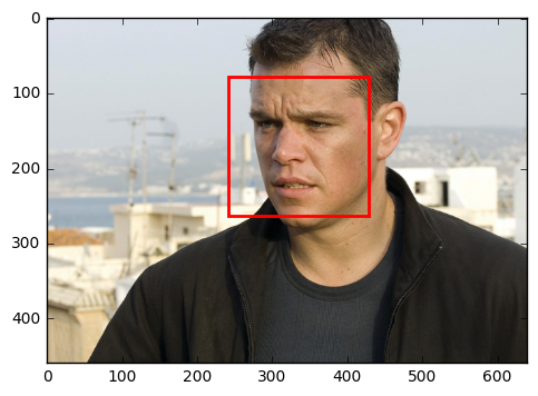
As you can see, using this library, you can get the bounding rectangle for a couple of lines of code. And the dlib detector, in contrast to OpenCV , works very well: from the entire base only a dozen faces it could not detect and did not create a single false response.
The formal formulation of our task implies that all individuals must be the same size. We will satisfy this requirement, at the same time aligning all faces so that the key points (eyes, nose, lips) are always in the same place of the image. It is clear that such a measure can help us regardless of the chosen mode of study and certainly does not harm. The algorithm is simple:
- There are a priori positions of key points in the unit square.
- Knowing the selected image size, we calculate the coordinates of these points on our image by simple scaling.
- Select the key points of the next person.
- We construct an affine transformation that takes the second set of points to the first.
- Apply an affine transformation to the image and trim it.
The reference position of the key points will be found in the examples to dlib (face_template.npy, download here ).
face_template = np.load(face_template_path) To find the key points on the image of the face, again, let's use dlib, using the already trained model, which can be found there, in the examples (shape_predictor_68_face_landmarks.dat, download here ).
predictor = dlib.shape_predictor(dlib_predictor_path) points = predictor(image, face_rect) landmarks = np.array(list(map(lambda p: [px, py], points.parts()))) Affine transformation is uniquely defined by three points:
INNER_EYES_AND_BOTTOM_LIP = [39, 42, 57] 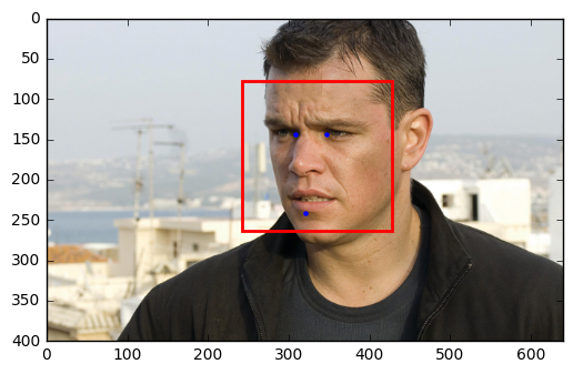
Let be
Find it:
proper_landmarks = 227 * face_template[INNER_EYES_AND_BOTTOM_LIP] current_landmarks = landmarks[INNER_EYES_AND_BOTTOM_LIP] A = np.hstack([current_landmarks, np.ones((3, 1))]).astype(np.float64) B = np.hstack([proper_landmarks, np.ones((3, 1))]).astype(np.float64) T = np.linalg.solve(A, B).T And apply to the image using the scipy-image library:
import skimage.transform as tr wrapped = tr.warp( image, tr.AffineTransform(T).inverse, output_shape=(227, 227), order=3, mode='constant', cval=0, clip=True, preserve_range=True ) wrapped /= 255.0 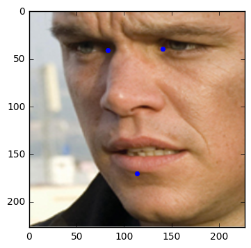
The full preprocessing code, wrapped in a convenient api, can be found in the preprocessing.py file.
The final chord of data preparation will be normalization: we calculate the average and standard deviation on the basis of the training and normalize each image on them. Do not forget about the development-set. See the code here .

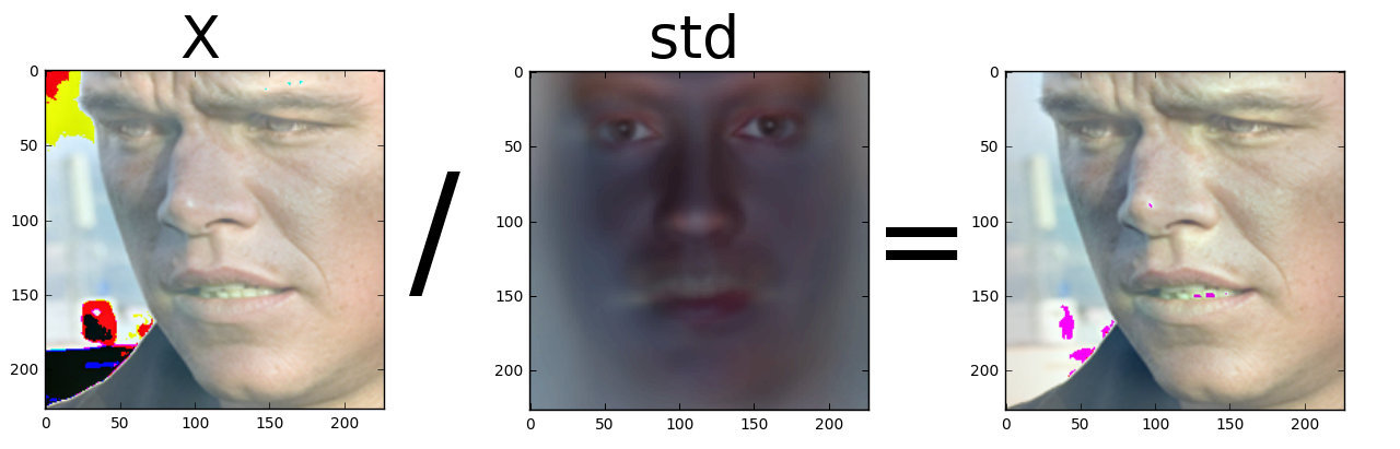
Collected, divided, aligned and normalized data can be downloaded here .
Bourne ultimatum
Data found and prepared, with a technique of testing sorted. Half the battle is done, the easiest is to find
Coin
Let's start the search from the very example of a bad function.
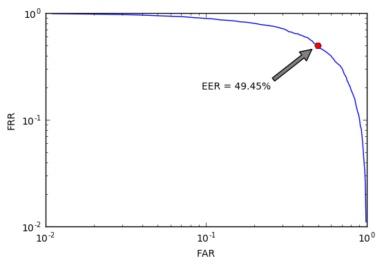

C EER = 49.5%, such an identifier is no better than a coin that we would toss when making each decision. Of course, this is understandable without graphs, but our goal is to learn how to solve identification problems and to be able to objectively evaluate any decisions, even obviously bad ones. In addition, it will from what to push off.
Distance
What is the function of two vectors from
Take, for example, the cosine distance:
And we will do all the same operations on the development-set:
dev_x = np.load('data/dev_x.npy') protocol = np.load('data/dev_protocol.npy') dev_x = dev_x.mean(axis=3).reshape(dev_x.shape[0], -1) dev_x /= np.linalg.norm(dev_x, axis=1)[:, np.newaxis] scores = dev_x @ dev_x.T tsc, isc = scores[protocol], scores[np.logical_not(protocol)] eer, fars, frrs, dists = calc_metrics(tsc, isc) We get this DET curve:

EER decreased by 16% and became equal to 34.18%. Better, but still not applicable. Of course, since we have so far only selected the function, without using the training set and machine learning methods. However, the idea is sensible with distance: let's leave it and present our function
Where
CNN
Great, you and I just made the task even easier. It remains only to find a good function.
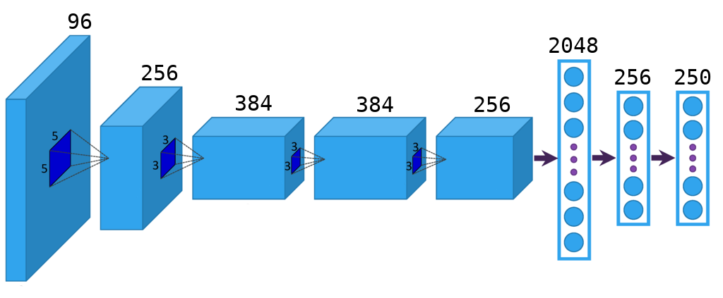
Model in keras
from keras.layers import Flatten, Dense, Dropout from keras.layers.convolutional import Convolution2D, MaxPooling2D from keras.layers.advanced_activations import PReLU from keras.models import Sequential model = Sequential() model.add(Convolution2D(96, 11, 11, subsample=(4, 4), input_shape=(dim, dim, 3), init='glorot_uniform', border_mode='same')) model.add(PReLU()) model.add(MaxPooling2D((3, 3), strides=(2, 2))) model.add(Convolution2D(256, 5, 5, subsample=(1, 1), init='glorot_uniform', border_mode='same')) model.add(PReLU()) model.add(MaxPooling2D((3, 3), strides=(2, 2))) model.add(Convolution2D(384, 3, 3, subsample=(1, 1), init='glorot_uniform', border_mode='same')) model.add(PReLU()) model.add(Convolution2D(384, 3, 3, subsample=(1, 1), init='glorot_uniform', border_mode='same')) model.add(PReLU()) model.add(Convolution2D(256, 3, 3, subsample=(1, 1), init='glorot_uniform', border_mode='same')) model.add(PReLU()) model.add(MaxPooling2D((3, 3), strides=(2, 2))) model.add(Flatten()) model.add(Dropout(0.5)) model.add(Dense(2048, init='glorot_uniform')) model.add(PReLU()) model.add(Dropout(0.5)) model.add(Dense(256, init='glorot_uniform')) model.add(PReLU()) model.add(Dense(n_classes, init='glorot_uniform', activation='softmax')) model.compile(loss='categorical_crossentropy', optimizer='adam', metrics=['accuracy']) And we will teach her to solve the classical classification problem on our training set: to determine which of the 250 subjects owns a face photo. Everyone knows how to solve such a simple task, in keras for this, besides the code above, you will need more lines 5-6. Let me just say that for the training base described in this article, it is vital to apply augmentation , otherwise there is not enough data to achieve good results.
You ask, what does the classification task have to do with it and how will its solution help us? Do it right! In order for the actions described below to make sense, it is necessary to make a very important assumption : if the network learns well to solve the classification problem in a closed set, then the penultimate layer of dimension 256 will concentrate all the important information about the face image, even if the subject was not in the training set .
This technique of extracting low-dimensional characteristics from the last layers of a trained network is widespread and is called bottleneck . By the way, the code for working with bottleneck in keras is located by reference .
The network was trained, 256-dimensional signs from the development-set were learned. We look at the DET- curve:

The assumption turned out to be true, reducing the EER by another 13%, reaching a result of 21.6%. Twice better than tossing a coin. Is it even better? Of course, you can build a bigger and more varied base, build a deeper CNN, apply various regularization methods ... But we are considering conceptual approaches, qualitative ones. And the amount can always be increased. I still have another trump card up my sleeve, but before putting it on the table, I’ll have to digress a little.
The Bourne Evolution

The key to improving our results lies in the realization that optimizing
The approach proposed by them was called TDE (Triplet Distance Embedding) and consisted of the following: let's build

Teaching such a network was suggested using triples.
which means that for a given anchor there is a gap between the spheres on which the positive and negative lies
Using this approach, the authors reduced the error by 30% on datasets Labeled Faces in the Wild and YouTube Faces DB , which is undoubtedly very cool. However, there is an approach and problems:
- it takes a lot of data;
- slow learning;
- additional parameter
which is not clear how to choose;
- in many cases (mainly with a small amount of data) it manifests itself worse than softmax + bottleneck .
This is where TPE (Triplet Probabilistic Embedding) comes on the scene - the approach described in Triplet Probabilistic Embedding for Face Verification and Clustering .
Why enter an extra parameter
It is simpler than the original and easily interpreted: we want the closest negative example to us to go further than the most positive positive example from us, but there should not be any gap between them. Due to the fact that we do not stop updating the network when the distance
We can calculate the probability that a triplet satisfies the given inequality:
Divide by
We will maximize the logarithm of probability, so the loss function will look like this:
And as a function

As you can see, this approach works better than the original one and has many advantages:
- less data required;
- extremely fast learning;
- no deep architecture required;
- can be used over existing and trained architecture.
We use this approach with you. All you need is 20 lines of code:
def triplet_loss(y_true, y_pred): return -K.mean(K.log(K.sigmoid(y_pred))) def triplet_merge(inputs): a, p, n = inputs return K.sum(a * (p - n), axis=1) def triplet_merge_shape(input_shapes): return (input_shapes[0][0], 1) a = Input(shape=(n_in,)) p = Input(shape=(n_in,)) n = Input(shape=(n_in,)) base_model = Sequential() base_model.add(Dense(n_out, input_dim=n_in, bias=False, weights=[W_pca], activation='linear')) base_model.add(Lambda(lambda x: K.l2_normalize(x, axis=1))) a_emb = base_model(a) p_emb = base_model(p) n_emb = base_model(n) e = merge([a_emb, p_emb, n_emb], mode=triplet_merge, output_shape=triplet_merge_shape) model = Model(input=[a, p, n], output=e) predict = Model(input=a, output=a_emb) model.compile(loss=triplet_loss, optimizer='rmsprop') If you want to use TPE in your projects, do not be lazy to read the original work, since I did not cover the main issue of training with triplets - the question of their selection. There is enough random choice for our small task, but this is the exception rather than the rule.
Let's train TPE on our bottleneck and take a look at the DET curve for the last time:

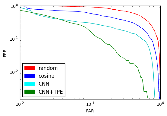
An EER of 12% is very close to what we wanted. This is twice as good as using CNN and 5 times better than random. The result, of course, can be improved by using a deeper architecture and a large base, but for the understanding of the principle and such a result is satisfactory.
Comparison of DET curves for all considered methods:
It remains to tie all kinds of machines and interfaces to our system, be it a web interface or an application on Qt, and the program for searching for identical faces in the photos is ready.

The application can be found on GitHub .
Thanks for reading! Put likes, subscribe to a profile, leave comments, learn machines good. Additions are welcome.
Literature
Source: https://habr.com/ru/post/317798/
All Articles