The logic of consciousness. Part 9. Artificial neural networks and minicolumns of the real cortex.

Veterinarian comes to the therapist. Therapist: - What are you complaining about? Veterinarian: - No, well, so everyone can!

Artificial neural networks are capable of learning. Perceiving many examples, they can independently find patterns in the data and highlight the signs hidden in them. Artificial neural networks in many tasks show very good results. The logical question is how neural networks resemble a real brain? The answer to this question is important mainly in order to understand whether it is possible, by developing the ideology of artificial neural networks, to achieve the same thing that the human brain is capable of? It is important to understand whether the differences are cosmetic or ideological.

Surprisingly, it is very likely that the real brain contradicts all the basic principles of artificial neural networks. This is doubly surprising, given that initially artificial neural networks were created as an attempt to reproduce just biological mechanisms. But the insidiousness of such situations. Very often, what seems plausible at first glance turns out to be the exact opposite of what it really is.

Artificial Neural Networks

Before describing the learning mechanisms of real neurons, we list the basic principles on which artificial neural networks are based. There are several of these principles. They are all very closely related. Violation of any of them breaks the whole concept of the work of artificial neural networks. After that, we will show that none of these principles is implemented in “true neural networks”.
')
Principle 1. Each neuron is a detector of a certain property.

A real neuron, if simplified to describe it, looks simple enough. On the dendrites are located synapses. Synapses are in contact with other neurons. Signals from other neurons through the synapses enter the body of the neuron, where they are summed up. If the sum exceeds a certain threshold, then a neuron's own signal arises - the spike, which is also the action potential. The spike extends along the axon and enters other neurons. Synapses can change their sensitivity. Thus, the neuron can be configured to respond to certain combinations of the activity of other neurons.

All of this, although it looks plausible enough, is very far from the work of real neurons. But for the time being we are describing a classic model and will follow this logic.

Simplified diagram of a real neuron

The formal model of the McCulloch-Pitts artificial neuron developed in the early 1940s follows inevitably from the above described (McCulloh J., W. Pitts, 1956).

McCulloch-Pitts Formal Neuron

The inputs of such a neuron signals. These signals are weightedly summed. Further, a certain nonlinear activation function, for example, sigmoidal, is applied to this linear combination. Often the logistic function is used as sigmoidal:



Logistic function

In this case, the activity of the formal neuron is recorded as

As a result, such a neuron turns into a threshold adder. With a fairly steep threshold function, the neuron's output signal is either 0 or 1. The weighted sum of the input signal and the neuron weights is a comparison of two images: the image of the input signal and the image described by the weights of the neuron. The result of the comparison is the higher, the more accurate the correspondence of these images. That is, the neuron, in fact, determines how much of the signal supplied is similar to the image recorded on its synapses. When the value of the weighted sum exceeds a certain level, and the threshold function switches to one, this can be interpreted as a neuron’s resolute statement that it has recognized the imaged image.

In different models there are various variations on how the artificial neuron should work. If we remove the threshold function, the neuron will turn into a linear adder. It is possible, instead of comparing with a template that sets weights, to check the input signal for compliance with the multidimensional normal distribution with certain parameters, this is used in networks based on radial basis functions. You can give signals distributed in time, and enter time parameters for synapses, thus setting the neuron for sensitivity to specific sequences. Other options are possible. The common thing between all of them is the correspondence of the neuron to the famous concept of “grandmother's neuron.

The key point for all neural networks is the perception of neurons as detectors of any properties. Something appears in the description - a neuron that corresponds to this “something” responds to it with its activity. Variations of neural networks are variations of the methods for detecting and teaching this detection.

Principle 2. Information in the neural network is a sign description.

In the classic view, each neuron sees a picture of the activity of other neurons that create its input signal. In addition, each neuron is a detector of something. If we collect the input signal into a vector, we get the so-called feature description .

In the attribute description, as the name implies, each element of the description vector corresponds to a specific attribute. It does not matter how the element is defined. This may be a binary value - a sign is present or not. There may be a quantitative value - how expressed is the sign in the description. Ordinal or nominal value - as this feature was realized in the description.

For example, take a binary 32-bit vector. We will encode the letters of the English alphabet.

First option. Zero bit - the letter "A", the first bit the letter "B" and so on. 26 bits will advise 26 letters. Then make a bit - capital letter or uppercase. Bit - italic or non italic, bit for thickness, bit for underline, and so on. If you encode one letter at a time, then you can encode one of the 26 letters in different spellings. This is a typical trait description. Every bit is a certain sign.

The second option. Machine coding, type, unicode. Characters are encoded with unique binary codes. But individual bits are no longer signs. In the codes of different letters not connected with each other there may be common units. Such coding is no longer an indicative description, although externally both there and there a 32 bit binary vector.

The information that neural networks deal with is always a trait description. And this follows from the first principle, according to which neurons are feature detectors.

Principle 3. A neural network, as a rule, is a converter of feature descriptions.

The input of the neural network is an indicative description. The result of the work is also an indicative description, but consisting of other features. For example, if we want to make a network that recognizes numbers by their image, then the input signs can be the brightness values ​​of the image points, and the output characters are recognized numbers.

When transforming one attribute description into another, it may be useful to use intermediate features that are not found in either the input or the output description. You can make several layers of such intermediate features. Such neural networks look like what is shown in the figure below.


Multilayer perceptron with two hidden layers (Heikin, 2006)

A typical example of a neural network with hidden signs is a layered network of direct distribution. Each layer of such a network, except for the input, consists of neuron detectors. These neurons are tuned to recognize certain signs. Each layer repeats the original description, but in its characteristic features of this layer.

If the output of the network is fed back to the input, then we obtain a dynamic recurrent network. In the forward propagation network, the output state is determined immediately after activation of all neurons. In a recurrent network, only with time does a steady state arise, which is the result of its work.

Regardless of the type of network on each layer, we are dealing with an attribute description made up of neuron detectors.

Principle 4. The number of neurons in a network determines the number of signs with which this network can operate.

The number of neurons on any layer of the network determines how many maximal signs are available to highlight this layer. Usually the number of neurons in the network is set initially before the start of training. Since it is not known in advance how many useful signs can stand out, the optimal number of neurons in the layers is selected iteratively.

In principle, it is possible, if necessary, to add new neurons on the fly, but this requires a special approach to training and is associated with significant difficulties.

Principle 5. Network training is the setting of the weights of the connections connecting neurons.

The detector of which property is one or another artificial neuron is determined by what values ​​take its weight. Training of the neural network occurs due to such a change in the weights of the neurons, which optimizes the requirements that we make to this network.

The two main types of learning are learning without a teacher and learning with a teacher.

Teaching without a teacher

When learning without a teacher, the neural network observes the input data, without having any idea in advance about which output signal should correspond to certain events. But since data may contain certain patterns, it is possible to adjust the behavior of the network in such a way that its neurons each respond to their own pattern.
For example, you can take a single-layer network consisting of linear adders and make it select the main components of the supplied data set . To do this, you can initiate a network with random weights, when giving a signal, determine the winner and then shift its weights in the direction of the given signal. As a result, the neurons themselves “drag” among themselves the main factors contained in the input information.

You can make an auto encoder . Create a network of three layers with the condition that the middle layer should be smaller than the input layer, and the output layer should be equal to the input layer. The task of the autocoder is to reproduce the pattern of the input layer as accurately as possible on the output layer.


Autocoder

Since there is a layer with a smaller dimension on the way from the entrance to the exit, the autocoder will have to learn how to compress the data, that is, select the most significant factors on the neurons of the middle layer. The middle layer in the future and will be the working output of the network.

For auto-coder training, you can read the error between the first and third layers at each step and adjust the network weights in the direction of reducing this error. This allows you to do, for example, the method of back propagation of error .

There may be other methods. For example, a network of radial basis functions , based on the ideas of the EM algorithm, can solve the problem of classification. In such a network, the neurons of the hidden layer do not evaluate the conformity of the supplied image and the image defined by the weights of the neuron, but the probability that the input signal corresponds to normal distributions, the parameters of which are stored in these neurons.

Teaching with a teacher

When training with a teacher, we determine in advance which output signal we want to receive from the network in each of the training examples. The task of training is to adjust the weights so that the network most accurately guesses the answers from the training set. Then there is hope that the network has caught patterns and will be able to guess the output signal for data that was not in the training.

For the direct distribution network, training is as follows. Initially, the network is initiated by random weights. A training example is provided and the network activity is calculated. An error is formed, that is, the difference between what should be on the output layer and what happened to the network. Further weights are adjusted to reduce this error.

For a single-layer perceptron, you can use the delta rule .
The delta rule is very similar to Hebb's rule, which has a very simple meaning: the connections of neurons that are activated together must be strengthened, and the connections of neurons that operate independently must weaken. But Hebb's rule was originally formulated for learning without a teacher and allows neurons to tune themselves to the allocation of factors. When learning with a teacher, joint activity should be understood somewhat differently. In this case, the Hebba rule takes the form:

• The first rule - If the output signal of the perceptron is incorrect and equal to zero, then it is necessary to increase the weights of those inputs to which the unit was applied.
  
• The second rule - If the output signal of the perceptron is incorrect and equal to one, then it is necessary to reduce the weights of those inputs to which the unit was fed.
  

If Y is the vector of the real output of the perceptron, and D is the vector that we expect to receive, then the error vector:


Delta rule for changing the connection between i and j neurons:



In fact, in a single-layer network, we are trying to build portraits of output features on neurons of the output layer in terms of input features. With weights of connections, we set the most characteristic, typical portrait of the output feature.

Difficulties begin when it turns out that an unambiguous portrait may not exist. For example, when we try to recognize letters, we can use both upper and lower case letters when learning. With this, if we do not make a difference between them, then the output neuron responsible for the letter “A” will have to respond immediately to two images - the image “A” and the image “a”. Similarly, the writing of letters can be completely different in different handwritings. If you try to combine all these portraits on one neuron, then nothing good will work. The image will be so blurred that it may be almost useless.

In such cases, a multilayer network with hidden layers helps. On the neurons of the hidden layers can be formed independent portraits of various realizations of the output signs. In addition, factors that are common to different output neurons can be distinguished in the hidden layers and are thus useful for differentiating one output feature from the other.

For teaching a multilayer network, the backpropagation method is used . The method consists of two passes: direct and reverse. With a direct pass, a training signal is given and the activity of all network nodes, including the activity of the output layer, is calculated. By subtracting the resulting activity from what was required to receive, an error signal is determined. During the back pass, the error signal propagates in the opposite direction, from the output to the input. At the same time, synaptic weights are adjusted in order to minimize this error.

Principle 6. Finite learning. Stability-plasticity dilemma.

When teaching a neural network, each time after submitting a new training example, a certain correction to the link weights is calculated. At the same time, gradients are calculated, which indicate in which direction this or that connection should be changed, strengthened or weakened.

At the beginning of training, you can behave quite boldly and relatively strongly correct the connections of neurons. But as far as learning, it turns out that abrupt changes are already unacceptable, as they begin to retrain the network, adjusting it to a new experience, while erasing the previous experience. The output is fairly obvious. The learning speed parameter is entered into the algorithms. As we learn, the speed decreases and the new experience no longer radically changes the weight, but only slightly corrects them.

The disadvantage of this approach is that, from a certain point in time, the network “stiffens” and ceases to change. For this reason, traditional networks are difficult to train. If such a need arises, it is easier to re-start from scratch to train the network on an extended data set that includes both old and new experiences.

The issue of additional training rests on the fact that the new experience begins to change the weights of the network and thereby changes the old training. The problem of the destruction of the old experience of new information is called the dilemma of stability-plasticity.

A solution is proposed by Stefan Grossberg (Grossberg, 1987) as the “theory of adaptive resonance”. The essence of this theory is that the incoming information is divided into classes. Each class has its own prototype - the image that most closely matches this class. For new information, it is determined whether it belongs to one of the existing classes, or whether it is unique, unlike any previous one. If the information is not unique, then it is used to refine the class prototype. If this is something fundamentally new, then a new class is created, the prototype of which lays down this image. This approach allows, on the one hand, to create new detectors, and on the other hand, not to destroy already created ones.

But the ideology of adaptive resonance is poorly compatible with other learning methods, since, in fact, requires the addition of new neurons directly in the process of learning the network.

Active Memory Learning Model

There are two approaches to learning - adaptive and batch. In adaptive learning, new experience is used to slightly change the previously achieved state of the weights of the network in order to adapt them to this new experience. In this case, it is assumed that the weights of the network already take into account all that is associated with previously acquired experience. In the batch approach, it is assumed that when receiving a new example, all previous experience remains available to us and when training we can not adapt the weights, but simply calculate them again.

Keeping previous experience greatly simplifies the issue of network stability-plasticity.
Consider the task of recognizing numbers, for example, the MNIST set. The images of handwritten numbers are fed to the input of the neural network, the output is monitored by the reaction of neurons corresponding to numbers from 0 to 9. The input images are 28 by 28 pixels in size, 784 points in total.


Example of handwritten numbers set MNIST

Usually, convolution networks and a multilevel architecture are used to solve such problems. We will consider the work of such networks in more detail later. Due to the simplicity and preliminary preparation of the MNIST kit (all figures are the same size and centered), good results are obtained even with a simple single-layer or double-layer perceptron.

The figure below shows the simplest single-layer network. The input of this network is 784 image points. Output - the neurons corresponding to the numbers.


Single-layer network for handwriting recognition

You can train such a network, for example, with a delta rule. As a result of training, the weights of the output neurons will tune into some averaged-schematic images of numbers. Blurred enough to “cover” their prototypes as much as possible, but not to “crawl” into other numbers. The learning speed parameter here has a very specific interpretation. Since a kind of averaging of images of a single digit occurs, the contribution of each following example to the formation of averaging should be inversely proportional to the number of examples that have already passed.

In the training set the same numbers are in a different spelling. For example, the deuce is “simple” and the deuce with a “loop” at the bottom (figure below). A simple network is nothing but to build a hybrid portrait, which, of course, does not improve the quality of its work.


Options "two"

In a multilayer network, there is a hope that in the hidden layers, the variants of the base of two are distinguished by separate features. Then the output layer will be able to more confidently recognize the two, focusing on the appearance of one of these signs.

Creating averaged blurred portraits allows you to successfully recognize images in most cases, but imposes a limit on the achievable quality of recognition. Blur inevitably leads to loss of information.

When learning the neurons of the output layer, “good” classifiers are created for each of the digits. Their weights are the best that can be obtained from the ideology of "let's make a portrait of a class."

When computers were weak or, God forbid, it was necessary to count manually, it was very important to use such methods that would allow to obtain good results with minimal calculations. Many ideas of "good" algorithms come precisely from such a saving of computations. It is necessary to make a certain discriminant function, which will allow to calculate the belonging of an object to a class.Or it is necessary to calculate the main factors and operate the description in them instead of the original data.

For any "good" basic algorithm, there is a limit of attainable accuracy, which is determined by what percentage of information was lost in the process of constructing factors or creating a discriminant function.

The overall result can be improved by using several different classifiers at once. From several classifiers it is possible to create a committee that will decide on the classification of an object by vote. This approach is called boosting .

When boosting, it is not necessary to use "good" classifiers. Any non-random, that is, those with a probability of correct assignment above the probability of a random choice, are suitable. The most interesting thing is that in many cases, by increasing the number of “bad”, but non-random classifiers, you can achieve an arbitrarily accurate result. Such reasoning is true for artificial neural networks.

The ideology of neuron-detectors trained in a blurry-averaged image is in many respects a tribute to the "economical" methods of calculation. True, learning itself is not always economical and fast, but the result is a network with a relatively small number of neurons.

An alternative to the concept of “good” neuron detectors may be the concept of “active memory”. Each individual learning example is an image that can independently act as a classifier. That is, for each teaching example, you can create a separate neuron, the weights of which will copy the input signal. Such a neuron can work, for example, in the linear adder mode, then its response will be the stronger, the more the supplied signal looks like the image it has memorized. From such detector memories, you can assemble the network shown in the figure below.


Neural network with memories-detectors. The connection between memories and output neurons is more complicated than just summation.

In the network shown in the figure, the input layer of neurons transmits its signal to the elements of the second middle layer. The elements of the second layer will not be called neurons, but called memories. Each teaching example creates a new memory. When setting the example, the newly created memory stamps on itself the exact image of the signal of the input layer. The output of the memory element closes at the neuron of the output layer corresponding to what the correct answer prescribes.

Teaching such a network with a teacher comes down to memorizing examples and creating example-response connections.

In recognition mode, each memory independently determines the degree of its similarity to the current image. From the cumulative triggering of memories, information is created for the output layer, which allows us to understand which neuron should be activated.

With the external simplicity of the network with memory, its operation is not as simple as it may seem. Elements of this network require significantly more complex logic of operation than from traditional formal neurons.

Comparison mechanism

The mechanism for comparing memories and images depends on the form of the description. It must be said that the indicative description is a rather unfortunate form. For example, two adjacent in the picture points in the attribute description give a zero match if the scalar product of the corresponding vector descriptions is used for comparison. It is for this reason that when encoding a picture through a vector describing the brightness of individual points, the “fuzzy” description is preferable to the “clear” one. In blurry pictures instead of a single point, a “spot” appears. Accordingly, close points start to give a certain match when comparing (figure below).


A single offset results in a complete absence of coincidence (left). A similar situation after blurring gives a significant coincidence (right) (Fukushima K., 2013)

The idea of ​​“blurring” is suitable not only for images, but also for any feature descriptions. To do this, you need to set the matrix of proximity signs description. Then, for any input signal before comparing, it is possible to create its “blurring” and use it already in a scalar product. For pictures, the proximity of features is determined by the proximity of points in the image. For arbitrary signals, specifying the proximity of features is somewhat more difficult. Sometimes the statistics of their joint manifestation can help.

«» «» «» , . , - «» , . .



MNIST , . . , , , .

When recognizing digits, it is necessary to estimate to which digit the current image is closer. To do this, you can calculate the average value of the match between the current image and the memories related to each of the numbers. Such an assessment of the averaged coincidence, although it will carry a certain meaning, will be bad for making a decision. For example, the class of twos contains at least two spellings - with and without the “loop” below. The situation is even worse, for example, with writing letters. Both uppercase and lowercase spellings of one letter can belong to one class.

In such cases, it is reasonable to average the examples separately for each of the spellings. That is, it makes sense to pre-cluster among the memories belonging to the same class, and divide them into appropriate groups.

, , . , «» , , . , MNIST , , , . , . , . , , , .



Each output neuron receives information about what memories are, in which there was something in common with the input signal, and information about the level of these coincidences. From this information it is necessary to conclude that there is a probability that we have the image for which the training took place. From the comparison of the probability for all output neurons, it is necessary to decide which of them is preferable and whether the level of the attained probability for the appearance of the output signal is sufficient.

Binary network output coding

, , . – ? , , – , .

Earlier we said that in the real brain, one minicolumn of the cortex, consisting of about one hundred neurons, performs the functions of a context computing module. That is, it analyzes what the information looks like in the context of this particular mini column. Each minicolumn has its own copy of memory and is able to conduct complete processing of information independently of the other minicolumns. This means that one minicolumn must perform all the functions that are characteristic of neural networks. At the same time, the number of signs that a minicolumn encounters is much more than a hundred and can be tens or hundreds of thousands.

One hundred neurons encode one hundred signs when talking about neuron detectors and feature descriptions. But we proceed from the fact that neurons do not form feature descriptions, but by their activity they create signals of a binary code that encode certain concepts.

It is easy to modify the neural network so that its output encodes not the indicative description, but the binary code of the feature. For this, it is necessary to “connect” the memories not with one output neuron, but with several forming the corresponding code. For example, digits from 0 to 9 can be encoded with a five-bit code so that each code contains exactly two units (figure below). Then each memory will affect not one, but two neurons. The result of such a network is not the activity of a single neuron corresponding to a digit, but a neural binary code of a digit. With such coding, neurons cease to be neurons of the grandmother, since their activity can manifest itself in completely different concepts.


Encoding the output of the network with a binary code

If we look at the network that was obtained as a result, it turns out that it already has little resemblance to traditional neural networks, although it fully retains all their functionality.

Let's look at the resulting network in the context of the previously formulated six principles of the classical neural network:

Principle 1. Each neuron is a detector of a certain property.
Not satisfied. The output neurons are not the grandmother's neurons. The same neuron is triggered by different signs.
Principle 2. Information in the neural network is a sign description.
Not satisfied. Network output is the concept code, not a feature set. The network input can also work with codes, and not with feature vectors.
Principle 3. A neural network, as a rule, is a converter of feature descriptions.
Not satisfied.
Principle 4. The number of neurons in a network determines the number of signs with which this network can operate.
Not satisfied. The output layer, containing a hundred neurons, when encoding a signal with ten active neurons, can display 1.7x10 ¹³ different concepts.
Principle 5. Network training is the setting of the weights of the connections connecting neurons.
Not satisfied. Memories are “linked” to neurons, but no adaptive change in weights occurs.
Principle 6. Finite learning. Stability-plasticity dilemma.
. . . . , « ». . , -.

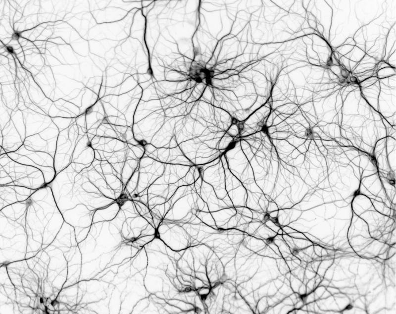
The main informational processes of our brain occur in its cortex. The cerebral cortex is divided into zones. Each zone consists of hundreds of thousands of minicolumns of the same structure. The number of neurons in a minicolumn, depending on the type of zone, is from 100 to 200. The

neurons of one minicolumn are located one under another. Most of their connections are concentrated in the vertical direction, that is, with the neurons of their own minicolumn.


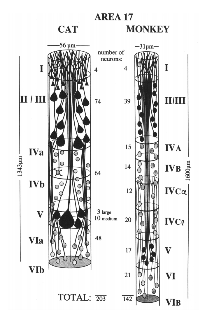
Minicolumns of the cat's primary visual cortex (left) and monkey (right) (Peters and Yilmaze, 1993).

It was previously assumed that each mini-column of the cortex corresponds to a different context. Minicolumns of any bark zone allow us to consider the same input information in all possible contexts for this zone and to determine which of them is better suited for the interpretation of the information received.

, , , . . . . , , .

. , . , «» .

As a result, a binary vector arises in each minicolumn, which is a description of how the source information looks in the context of a minicolumn.
From this point on, what happens in every minicolumn is a lot like the behavior of the memory network just described.

Fixing the feature code

In order for the minicolumn to work with the memory network mechanism, it is necessary to show how to remember the binary vector of the description and how to link this memory with the code of the corresponding feature.

In our biological model, memory is a kind of fixation of the “interference” of two patterns. Earlier, it was shown how to memorize the pairs “identifier - description”. Now we need to remember a pair of "code of the sign - description." The trait code is a combination of the activity of neurons of a minicolumn. Description is the activity of dendritic segments inside the same mini-column. To fix the interference of two patterns is to memorize the pattern of the second pattern on the elements of the first pattern.

Suppose that somehow we managed to “tag” the neurons that form the trait code. Then, in order to fix a memory of the type “attribute code - description” it is necessary to memorize the description picture on each of the marked neurons.

– , . . . – . .

We will not try to guess in detail how the process of memorization proceeds, we will describe its ideology. The description signal triggers the release of neurotransmitters in certain synapses related to the minicolumn. It is possible that this happens through the creation of a hash that causes the activity of a part of the neurons. It is possible that other mechanisms will be involved. Now it does not matter. Just assume that the pattern of dendritic activity led to a picture of the release of neurotransmitters. Moreover, the ejection picture turned out to be strictly dependent on the information picture. This means that different informational patterns create different patterns of neurotransmitter emission distribution. The conversation is about neurotransmitters and modulators that fall into extra-synaptic space.

, , . . .

For any signal such places in the minicarrier will be many. So with a probability close to one, at least one such place exists on each dendritic segment. This means that there will be several dozen of such places on the dendrite of one neuron. But each of the places will not be sensitive to the whole signal, but only to its specific fragment. If we present an information signal with a binary vector, then one chosen place is a place that reacts not to the whole vector, but to several specific significant bits of this vector. The figure below shows an example when each of the selected places highlighted in red captures four of the nine active bits in the input signal.


Places on the dendrite surface of a single neuron selected with respect to a specific signal.

To fix the memory on a selected neuron, it is necessary to take clusters of receptors sensitive to the combination of mediators that have arisen there, and place them in the "active" state. The active state implies that from now on, if the neurotransmitter release pattern recurs, the receptor cluster will recognize this and open the nearby ion channel, resulting in a miniature excitatory postsynaptic potential in this place. In other words, the repetition of the signal will cause a small, of the order of 1 mV, shift of the membrane potential towards the excitation side. This shift will be a point and will affect only the chosen location.

. , , . . , .

, , . , .

. , . , , 15 100, 15 , . , , .

ABC, ( ).


Binary codes of three concepts and total binary code

Each of the selected places captures the trace of not the entire signal, but only its random fragment. This means that among the selected places there may be places that are more sensitive to the combination of any part of the source code attributes.

Now suppose that we have given a signal containing only two signs AB. Its code will be as shown below.

Binary codes of two concepts and total binary code

For the same neuron that was at the beginning, a new signal will give only one selected place. In the image below, it is highlighted in red. This location will be common to AB and ABC signals. Creating an AB signal there will cause the response to any signal containing AB to be stronger at this location than in other selected locations.

Reduction of the reaction of selected sites for a partial signal

As a result of such combinatorial memorization, it turns out that if the incoming signals contain patterns, that is, stable combinations of features, then there may be places into which “partial” memories associated with these combinations will start to fall. Such places can be called resonant points.

The more often in different examples with the same training code there is a certain combination of signs, the more memories will be in the corresponding resonance point and the more active its reaction will be. Memories from ABD, ABFG, and the like will fall into the resonance point corresponding to the signal AB.

, . «» , , .

, , . , . , , .

, , , , . , , , , . , .

, , , , . , .

In the process of learning with the teacher, the input images are supplied to the network input and it is indicated what output signal we want to receive. As experience is gained, the network can identify patterns in the input data and compare them with output features. But this only works if the input descriptions can be “normalized”. Before looking for patterns, it is required to bring all input descriptions to a “common denominator”. If we are dealing with images, then before attempting to compare them, it is necessary to convert them to a common scale, rotation and find an offset at which the desired images in different examples will coincide as much as possible. In the classical approach, this is solved using a convolutional layer; we do this using the context space. That is, before memorizing a new “two”, you first need to transform it so that it coincides as much as possible with the previous “two”.

When a context is found in which a new description is consistent with previous experience, we say that the interpretation in this context implements the meaning of the information. It is in this interpretation that the memory of this experience is created. This applies not only to visual, but also to any other information. Such a memory is convenient in that when it is “superimposed” on previous memories, the common between them appears.

Since a copy of the same memory must be kept in all contexts, when the necessary interpretation is in one of the contexts, it must also be remembered in all the others. In the real crust, this means that at the moment of memorization, all contexts will have to “abandon” their own interpretations, reproduce the chosen interpretation and remember it. If there is training with the teacher and the required code of the characteristic is known, then remember with this code.

Earlier we said that organizing the context space requires that each minicolumn keep the transformation rules not only for its own, but also for all other contexts. This allows you to move minicolumns simply by changing the pointer to which context the minicolumn should be used. Such a total memory for transformations allows realizing not only the movement of contexts, but also synchronous memorization.

For memorization, it is enough that the code of the context in which the meaning of the information is determined and the characteristic code required for learning is spread throughout the cortex. Then each minicolumn can independently reproduce the necessary interpretation and perform memorization.

In this section, we have considered a learning mechanism with a teacher that is possible for the cortex. This mechanism is quite simple, as is the very simple formulation of the problem - by examples learn how to correctly assign objects to the desired class. The task of self-learning is much more interesting and more complicated - there are data, there are patterns in them, it is required to single out these patterns. The difficulty is that in the brief statement of the problem nothing is said about what patterns we are interested in, how many patterns need to be highlighted, whether we are interested in particular rare patterns or whether we need to look for the most general rules, whether we want to build an orthogonal basis or whether we are satisfied with the description in oblique factors. The next part will talk about what a universal solution the brain can offer to solve this problem.

Alexey Redozubov

The logic of consciousness. Part 1. Waves in the cellular automaton
The logic of consciousness. Part 2. Dendritic waves
The logic of consciousness. Part 3. Holographic memory in a cellular automaton
The logic of consciousness. Part 4. The secret of brain memory
The logic of consciousness. Part 5. The semantic approach to the analysis of information
The logic of consciousness. Part 6. The cerebral cortex as a space for calculating meanings.
The logic of consciousness. Part 7. Self-organization of the context space
The logic of consciousness. Explanation "on the fingers"
The logic of consciousness. Part 8. Spatial maps of the cerebral cortex
The logic of consciousness. Part 9. Artificial neural networks and minicolumns of the real cortex.
The logic of consciousness. Part 10. The task of generalization
The logic of consciousness. Part 11. Natural coding of visual and sound information
The logic of consciousness. Part 12. The search for patterns. Combinatorial space