Performance comparison of GPU calculations in Python and C

Python has a number of attractive advantages, which include ease of implementation of software solutions, clarity and conciseness of the code, the presence of a large number of libraries and numerous active community. At the same time, the well-known slowness of the python often limits its applicability to "heavy" calculations. For a number of tasks, it is possible to achieve a significant acceleration of calculations by using the CUDA technology for parallel computing on the GPU. The purpose of this small study is to analyze the possibilities of effectively using python for calculations on GPU and comparing the performance of various python solutions with implementation on C.

Introduction

By the nature of my work, I often do numerical modeling tasks. In many cases, we use CUDA technology to speed up calculations by using the parallel computing capabilities of the GPU, while programs are written in C. At the same time, in some cases, we would like to be able to implement calculations on python, because it is convenient, fast , flexible, concise, youth . In this case, however, it is very important not to lose the speed of program execution, since some calculations can take from several hours to a day. The article demonstrated the use of the python-libraries Numba and PyCUDA for the implementation of parallel calculations on the GPU and the results of the comparison of their performance on the test task.

Test task

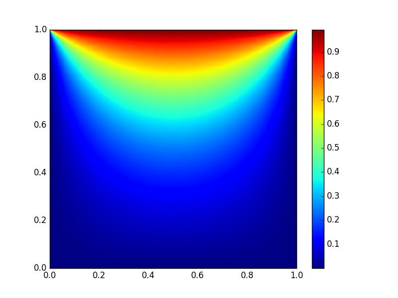
The choice of the test problem and the conditions of testing was determined by the nature of the real problems, for which further use of python is planned. In this case, the simplest problem was chosen, namely the problem of solving the two-dimensional heat conduction equation using an explicit finite-difference scheme . The task was considered on a square domain with given temperature values ​​at the boundaries. The number of nodes of the computational grid in x and y is the same and is equal to n. The figure at the beginning of the article shows the steady-state solution to the test problem.

Algorithm and testing conditions

The algorithm for solving the problem can be represented by the following pseudocode:
')

  u0  u,                   u0  u     for(i = 0; i < nstp/2; i++)   u     ,   u0       u0     ,   u       (u0)          

In all tests presented below, the number of square grid nodes in each direction (n) ranged from 512 to 4096, and nstp = 5000.

Software and hardware

Testing was conducted on a personal computer:

Intel® Core (TM) 2 Quad CPU Q9650 @ 3.00GHz, 8 Gb RAM
GPU: Nvidia GTX 580
Operating system: Ubuntu 16.04 LTS with CUDA 7.5 installed

C implementation

All further python implementations were compared with the results obtained using the C program described in this section.


Calculations show that for N = 512, the execution time of the C program parallelized on the GPU is 0.27 seconds versus 33.06 seconds for the sequential implementation of the algorithm on the CPU. That is, the CPU / GPU acceleration is about 120 times. With increasing N, the magnitude of the acceleration does not decrease.

Python with Numba

The Numba library provides the ability to jit (just-in-time) compile python code into byte-code comparable in performance to C or Fortran code. Numba supports compiling and running python code not only on the CPU, but also on the GPU, while the style and appearance of the program using the Numba library remains purely Python.


Note here are some nice features. First, this implementation is much shorter and clearer. Here we used two-dimensional arrays, which makes the code much more readable. Secondly, if in the C-implementation we were required to pass all constants (for example, N) by executing functions like cudaMemcpyToSymbol(dN, &N, sizeof(int)); here we simply use global variables as in the usual python functions. Finally, the implementation does not require any knowledge of the C language and the GPU architecture.

This code is easy to rewrite and for the case of using one-dimensional arrays of size n * n, as will be shown later, this significantly affects the execution speed.

PyCUDA

The second python library tested was the PyCUDA library. Unlike Numba, here from the developer you will need to write kernel code in C, therefore you cannot do without knowledge of this language. On the other hand, apart from the actual C kernel, you do not need to write anything.


This all looks like a pure python with the exception of a local C-code insert.

Performance comparison

Figure 1 and Table 1 show the dependencies of the test program runtime (in seconds) on the mesh size n, obtained when running the C code (CUDA C curve) and python implementations with the Numba library and two-dimensional arrays (Numba 2DArr), with the library Numba and one-dimensional arrays (Numba 1DArr), with the PyCUDA library (PyCUDA curve).


Picture 1

Table 1

n	Cuda c	Numba 2DArr	Numba 1DArr	PyCUDA
512	0.25	0.8	0.66	0.216
1024	0.77	3.26	1.03	0.808
2048	2.73	12.23	4.07	2.87
3073	6.1	27.3	9.12	6.6
4096	11.05	55.88	16.27	12.02

Figure 2 shows the relationship between the execution times of various python implementations and the execution time of the C code. As can be seen from the figures, the slowest of the considered is the implementation using the Numba library using two-dimensional arrays. At the same time, this approach is the most obvious and simple. Interestingly, the sweep of two-dimensional arrays in one-dimensional leads to approximately threefold acceleration of the code. The quickest solution was to use the PyCUDA library. At the same time, as noted above, using this library is somewhat more laborious, since it requires writing a kernel in C. However, the costs pay off and the execution speed of such a python program is only 5-8% less than a program written entirely in C.


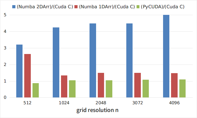
Figure 2

findings

Miracles do not happen and the most simple and visual solutions are at the same time the slowest. At the same time, the available libraries allow you to achieve the speed of execution of python-programs, comparable to the speed of execution of pure C-code. Existing libraries give the developer a choice between more and less high-level solutions. This choice, however, there is always a trade-off between the speed of development and the speed of program execution.

Links

» Numba Library Documentation
» Examples of using Numba
» PyCUDA Library Documentation
» PyCUDA usage examples