Prediction of the severity of insurance claims for Allstate. Graduation project of our graduate
Habr, hello! Our graduate of the 4th recruitment of the Big Data Specialist program , Kirill Danilyuk, shared his research, which he carried out as a final project in one of the courses. All the documentation and description is on his githaba . Here we provide a translation of his report. Caution - Longrid.
Many people working in data-related areas have heard of Kaggle, the platform for data science competitions. Today, more than 600 thousand data scientists and many well-known companies are represented at Kaggle. The company describes its problem, sets quality metrics, publishes a set of data that could help solve it, and participants find original ways to solve the problem posed by the company.
This Kaggle competition is sponsored by Allstate, the largest publicly traded company in the United States in the personal and life insurance business. At the moment, Allstate is developing automatic methods for predicting the cost (severity) of insurance claims and has asked the Kaggle community to demonstrate fresh ideas and new approaches to solving this problem.
The company seeks to improve the quality of its services in processing insurance claims and has published a set of data on accidents that have occurred in households (each household is represented by an anonymized feature vector) with a numerical estimate of the value of the insurance claim. Our task was to predict the severity of a possible insurance claim for a new household.
')
Several more data sets related to this task are also available on Kaggle:
• Allstate insurance claims prediction competition - an earlier Allstate competition, the purpose of which was to predict insurance premiums based on the characteristics of the insured vehicle. The data set of this competition provides an opportunity to dive into the insurance field.
• The fire loss assessment competition is a competition held by the Liberty Mutual Group and aimed at predicting the expected fire losses to form the terms of insurance contracts. This is another example of a data set from the insurance industry that helped us gain an understanding of the approaches to solving prediction problems in the insurance industry.
Separately, I note that the original data set is highly anonymous (both in terms of the names of features and in terms of values). This aspect complicates both the understanding of the meaning of the signs and the enrichment of the data set from external sources. Competitors tried differently to enrich and interpret the original data, but the success of their attempts remains controversial. On the other hand, there seems to be no data leakage in this data set, which occurs when additional information remains in the training data. Such information can be highly correlated with the target variable and lead to unreasonably accurate predictions. Recently, a large number of Kaggle competitions have suffered from such leaks.
We have at our disposal a data set containing records for the insurance claims of Allstate’s customers. Each entry contains both categorical and continuous signs. The target variable is a numerical estimate of the losses caused by this insurance claim. All signs are made as anonymous as possible: we do not know either the real names of the signs or their true meanings.
Our goal is to build a model that will be able to predict future losses correctly on the basis of given values of attributes. Obviously, this is a regression task: target variable is numerical. This is also the task of teaching with the teacher: the target variable is clearly defined in the training data set, and we need to get its values for each record of the test set.
Allstate did a great job of cleaning and preprocessing the data: the data set provided is very clean and (after some additional processing) can be transferred to a large number of learning algorithms with the teacher. As we will see in the part of the data research report, the task of Allstate does not specifically allow generating new features or preprocessing existing features. On the other hand, this datasset pushes the use and testing of various machine learning algorithms and ensembles - just what is needed for a graduation project.
I applied the following approach to the Allstate project:
1. Investigate the data set, understand the meaning of the data, the characteristics and the target variable, and find simple relationships in the data. This step is performed in the Data Discovery notebook file .
2. Perform the necessary data preprocessing and train several different machine learning algorithms (XGBoost and multilayer perceptron). Get baseline results. These tasks are solved in the XGBoost and MLP files.
3. Adjust the models and achieve a noticeable improvement in the results for each of them. This step is also implemented in the XGBoost and MLP files.
4. Train the ensemble using the overlaying technique of models (stacking) using the previous models as basic predictors. Get the final results that will be significantly better than the previous ones. This stage is implemented in the Stacking notebook file.
5. Briefly discuss the results, assess the final position in the tournament standings and find additional ways to improve it. We’ll talk about the results below in this report and in the last part of the Stacking notebook file.
The Kaggle platform requires the company conducting the competition to clearly define the metrics on which participants can compete. Allstate chose MAE as such a metric. MAE (mean absolute error) is a very simple and obvious metric that directly compares the predicted and true values.

This metric is set and cannot be changed, because is part of the competition conditions. Nevertheless, I consider it well suited to this task. Firstly, MAE (as opposed to MSE or RMS error) does not give a large penalty for an incorrect estimate of emissions (there are several emissions with abnormally high loss values in the data sheet). Secondly, MAE is easy to understand: error values are expressed in the same dimensions as the target variable itself. Generally speaking, MAE is a good metric for beginners in data science. It is easy to compute, easy to understand, and difficult to misinterpret.
For a complete acquaintance with this stage, you can refer to the Data Discovery file.
The entire training sample consists of 188318 elements indexed by the variable uid. The index for working with data does not carry additional information, since it's just a numbering, starting with “1” with some missing values. We are not going to use a test set without an index for prediction (it is necessary to send results to Kaggle), however it is worth noting that the test data set is organized in the same way as the training set. Obviously, the training and test samples were obtained from one data set by a partitioning procedure, for example, train_test_split from the sklearn package.
The main results of this part of the project are as follows:
• The data set contains 130 different signs (without taking into account the id index and the target loss variable). Given the size of the data set, this is quite a reasonable number of signs. We could hardly face the "curse of dimension" here.
• 116 signs categorical, 14 numerical. We will probably need to encode these 116 features, since most machine learning algorithms cannot correctly handle categorical variables. We will discuss the ways of such coding and the differences between them later.
• There are no missing values in the entire data set. This fact only confirms that Allstate provided data with a high degree of preprocessing in order to make it accessible and easy to use.
• Most categorical features (72 or 62%) are binary (yes / no; male / female), but their meanings are written simply as “A” and “B”, so we cannot guess their meaning at all. 3 signs take three different values, 12 signs - 4 different values.
• Numerical signs are already scaled in the range from 0 to 1, standard deviations for all of them are close to 0.2, average values are about 0.5, therefore we cannot make any assumptions about their values for these signs.
• Apparently, some numerical traits used to be categorical before they were converted to numerical traits using LabelEncoder or a similar procedure.
• By constructing histograms of various signs, you can make sure that none of them obeys the normal distribution law. You can try to reduce the asymmetry of the distribution of these data (in the case of scipy.stats.mstats.skew> 0.25), but even after such a conversion, it will not be possible to achieve a distribution that is close to normal.
• The target variable is also not normally distributed, although it can be reduced to a normal distribution by a simple logarithmic transformation.
• The target variable contains several outliers with abnormally high values (very serious incidents). Ideally, we would like our model to be able to identify and correctly predict such outliers. At the same time, we can easily retrain them if we are not careful enough. It is clear that some compromise is needed here.
• The training and test samples have similar data distributions. This is an ideal breakdown characteristic for training and test samples, which greatly simplifies cross-validation and allows us to make informed decisions about the quality of models using cross-validation in the training data set. This greatly simplified participation in the Kaggle competition, but it would not be useful to complete the graduation project.
• Several continuous features are highly correlated (the correlation matrix is shown in Fig. 1 below). This leads to data-based multicollinearity in this data set, which can drastically reduce the predictive ability of linear regression models. Part of this problem can be solved with L1 or L2 regularization.
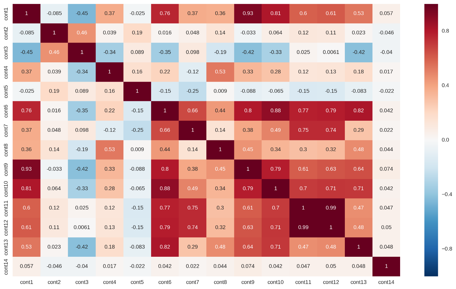
Figure 1: Correlation matrix for continuous features
I will show one visualization in order to demonstrate an important feature of this data set - a high degree of anonymity, preprocessing of data.
Below are histograms of 14 continuous signs labeled as cont #. As can be seen from fig. 1, the data distributions may have multiple peaks, and the density functions of the distributions are not close to Gaussian. We could try to reduce the data asymmetry factor, but the use of normalization algorithms (for example, the Box-Cox transform) did little for this data set.
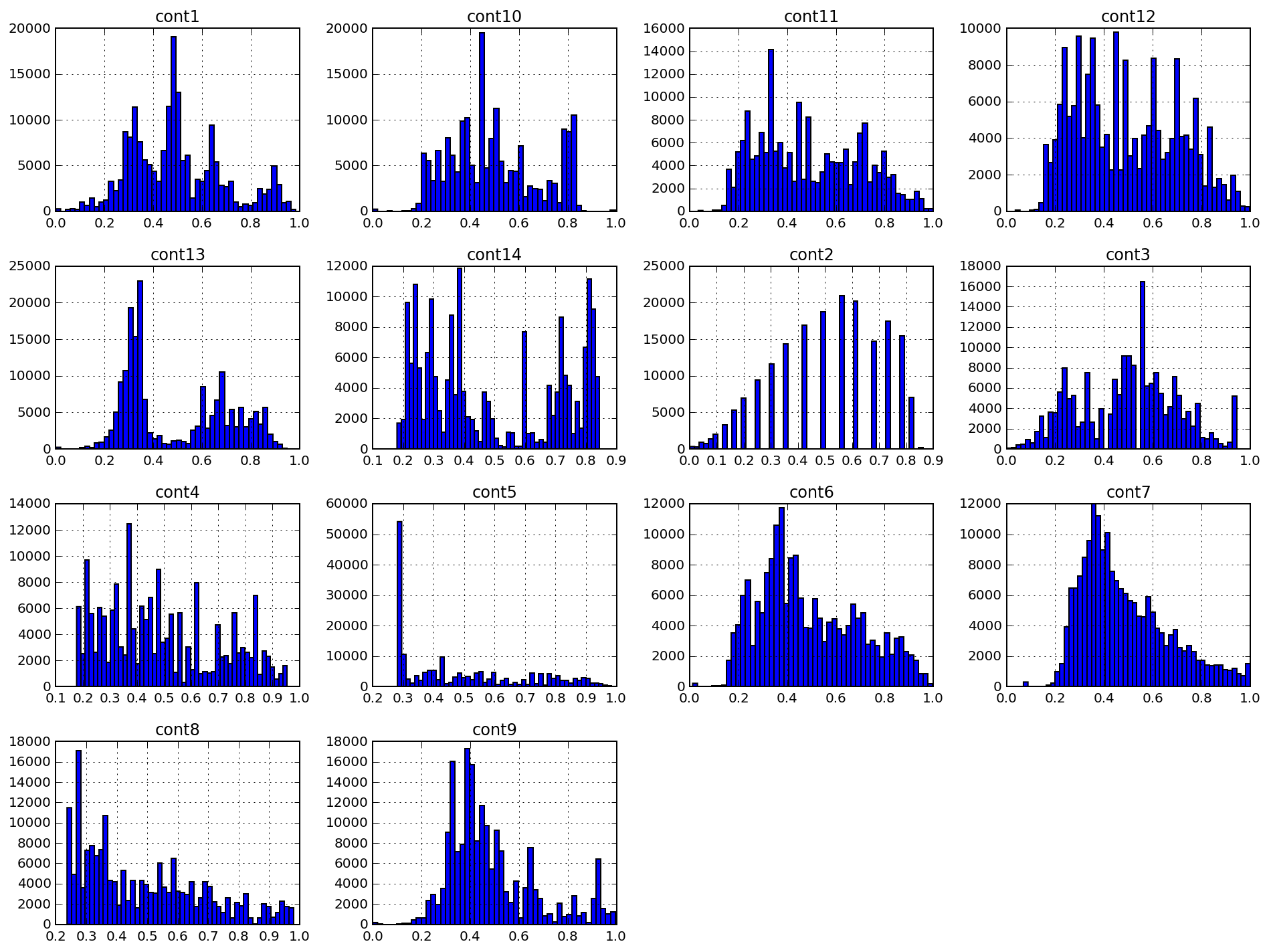
Figure 2: Continuous features histograms
The cont2 feature is especially interesting. This feature was apparently derived from the categorical and may reflect the age or age category. Unfortunately, I did not go deep into the study of this feature: he had no influence on my project.
This section is much more detailed in the following two documents: XGBoost notebook and MLP notebook .
XGBoost. One of the reasons for my interest in the project is the opportunity to try the method of boosting over trees and, in particular, XGBoost. De facto, this algorithm has become a kind of standard Swiss knife for many Kaggle competitions due to its scalability, flexibility and impressive predictive power.
XGBoost is suitable for teacher learning tasks similar to the one we have (clearly defined training data set and target variable). Below we describe the principles of the XGBoost algorithm.
XGBoost, in essence, is a variation of boosting — an ensemble meta-algorithm for machine learning, used to reduce bias and variance in teacher training, and a family of machine learning algorithms that turn weaker models into stronger ones. Source: Wikipedia . Initially, the ideas of boosting are rooted in the question posed by Kearns and Valiant, whether “weak” learning algorithms that give results a little better than random guessing in a PAC (probably approximately correct) model, can be “strengthened” to a “strong” learning algorithm arbitrary accuracy. Source: A brief introduction to boosting (Yoav Freund and Robert E. Schapire). An affirmative answer to this question was given to RESchapire in his article The Strength of Weak Learning , which led to the development of many boosting algorithms.
As you can see, the fundamental principle of boosting is the consistent application of weak learning algorithms. Each successive weak algorithm attempts to reduce the displacement of the entire model, thus combining weak algorithms into a powerful ensemble model. Many different examples of algorithms and methods of boosting can be given, such as AdaBoost (adaptive boosting, which adapts to weak learning algorithms), LPBoost and gradient boosting.
XGBoost, in particular, is a library that implements a gradient boosting scheme. Gradient boosting models are built in stages, just as with other boosting methods. This boosting method generalizes weak learning algorithms, allowing optimization of an arbitrary differentiable loss function (loss function with a computable gradient).
XGBoost, as a kind of boosting, includes an original decision tree-based machine learning algorithm suitable for working with sparse data; theoretically sound procedure allows you to work with weights of various elements in the training of trees. Source: XGBoost: scalable tree-boosting system (Tianqi Chen, Carlos Guestrin)
There are several advantages of the XGBoost algorithm:
• Regularization. As will be shown in the section on the model of a multilayer perceptron, using other algorithms one can easily obtain a retrained model. XGBoost provides very reliable ready-to-use regularization tools along with a set of parameters to customize this process. The list of these parameters includes: gamma (the minimum reduction of the loss function required for further tree division), alpha (weight for L1 regularization), lambda (weight for L2 regularization), max_depth (maximum depth of the tree), min_child_weight (minimum sum of all weights observations required for the child).
• Implementation of parallel and distributed computing. Unlike many other boosting algorithms, training here can be done in parallel, thereby reducing training time. XGBoost works really fast. According to the authors of the aforementioned article, “the system works more than 10 times faster than existing popular solutions already on one computer and can be scaled to millions of copies in a distributed or memory-limited environment.”
• Integrated cross-validation. Cross-validation is a prerequisite for assessing the quality of the resulting model, and in the case of XGBoost, its process of working with it is extremely simple and straightforward.
MLP. The second model we are building is a fully connected direct propagation neural network or a multilayer perceptron. Since our ultimate goal is to build an ensemble (stacking) of basic regressors (and we decided on the type of the first one, XGBoost), we need to find another “type” of a generalizing algorithm that will otherwise examine our data set.
This is when they mean when they say that generalizing algorithms of level zero should “cover space”. Wolpert, Generalization overlay.
By adding more layers and more elements within each layer, the neural network can capture very complex non-linear connections in the data. The universal approximation theorem states that a direct propagation neural network can approximate any continuous function in Euclidean space. Thus, the multilayer perceptron is a very powerful simulation algorithm. Multilayer perceptrons are easily subject to retraining, but we have all the necessary tools at our disposal to reduce the influence of this factor: accidental deactivation of neuron activation (dropout), L1-L2 regularization, packet normalization (batch normalization), etc. We can also train several similar neural networks and average their predictions.
The deep learning community has developed high-quality software for learning and evaluating models based on artificial neural networks. My models are based on TensorFlow , a library for tensor computing developed by Google. To simplify the construction of models, I decided to use Keras , a high-level front end for TensorFlow and Theano, which takes over most of the standard operations needed to build and train neural networks.
GridSearch and Hyperopt. These methods are used to select models and configure hyperparameters. While the GridSearch (grid search) exhaustively enumerates all possible combinations of parameters, Hyperopt either selects a given number of candidates from the parameter space with a given distribution, or uses a form of Bayesian optimization. Together with both of these selection methods, we use a cross-validation technique to assess model performance. We use cross-validation with splitting into k parts (k-fold) with three or five parts depending on the computational complexity of the model.
Overlay models (stacking). We combine the predictions of two of our models (XGBoost and the multilayer perceptron) to construct the final prediction using a meta-regressor. This method is called stacking and is used extensively on Kaggle (often excessively). The idea of stacking is to split the training sample into k parts and train each of the basic regressors into k-1 parts, making predictions for the rest. As a result, we get a training sample with regressor predictions (out-of-fold), while having real values of the target variable. Next, we train the metamodel on this data, using the predictions of each regressor as a sign for the metamodel, and the true values as the target sign.
To the trained metamodel, we input the regressor prediction for the test sample and we get the final predictions in which the trained model takes into account the characteristic errors of each regressor. The implementation of this stage is described in detail in the Stacking notebook file .
The first result was given by Allstate: they trained an ensemble model of a random forest and got the result MAE = 1217.52141. This result is easily surpassed even by a simple XGBoost model, and most of the participants succeeded.
I also set several criteria for myself when I was teaching models. The bottom line for me was the performance of a simple model of this class. For XGBoost, this result was set to MAE = 1219.57, it is achieved by a simple model of 50 trees without any optimization or adjustment of the hyperparameters. I took the standard values of the hyperparameters (suggested in the article from Analytics Vidhya ), left a small number of trees and got this starting result.
For a multilayer perceptron, the performance of a two-layer model with a small number of elements in its hidden layer (128) with the ReLU activation function, standard initialization of weights and the Adam GD optimizer: MAE = 1190.73 was chosen as the baseline result.
In this thesis project, I avoided complex baseline-models, because I understand that all the results should be reproducible. I also participate in this Kaggle competition, but learning all my models used in the competition, most of which are combinations and uses a large number of algorithms, will definitely require too much time from the reader. In the Kaggle competition, I hope to surpass the result of MAE = 1100.
I already mentioned that this dataset was already well prepared and pre-processed, for example, continuous attributes were scaled to the interval [0,1], categorical attributes were renamed, their values were turned into numbers. In fact, in terms of preprocessing, there is not much left that could be done. However, some work still needs to be done in order to train the correct models.
Target variable pre-processing
Our target attribute has an exponential distribution, which can lower the quality of regression models. As you know, regression models work best when the target variable is distributed normally.
To solve this problem, we simply apply a logarithmic transformation to the target variable loss: np.log (train ['loss']).
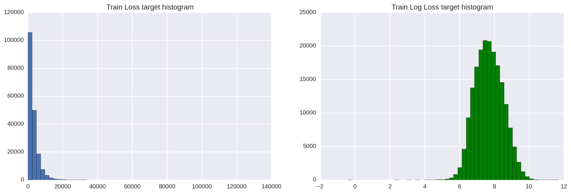
Figure 3: Histograms of the distribution of the target variable before and after the logarithmic transformation
The result can be improved: to the left of the main distribution bell several deviating observations lie. To get rid of these emissions, we can shift all the values of the loss variable by 200 points to the right (loss + 200) and then take the logarithm from them.
Coding categorical variables
Most machine learning algorithms cannot directly work with categorical variables. XGBoost is no exception here, so we will need to convert our categorical variables to numeric ones. Here we can choose one of two standard strategies: label coding (label encoding) or direct coding (one-hot encoding). What strategy to use is a rather controversial question, but here several factors should be considered:
Directly encoding (one-hot encoding) is the basic way of working with categorical features. It produces a sparse matrix, where each new column represents one possible value of a single feature. Since we have 116 categorical variables, and the variable cat116 takes 326 values, we can get a sparse matrix with a huge number of zeros. This will lead to longer training, increase memory costs and may even worsen the final results. Another disadvantage of direct coding is the loss of information in cases where the order of categories is important.
Label encoding , on the other hand, simply normalizes the input data column so that it contains only values between 0 and the number of classes -1. For many regression algorithms, this is not a very good strategy, but XGBoost can cope and does this transformation very well.
For XGBoost we will use LabelEncoder and normalize the input data. For a multilayer perceptron, we will need to create dummy variables, so our choice here is one-hot encoding.
As mentioned earlier, our methodology for implementing machine learning will be divided into two sections:
• Training, tuning, and cross-validation of base models (zero-level models): XGBoost and multilayer perceptron, assuming that we have already made preliminary data preparation, which is slightly different for these two models. The difference will be in the coding of the signs (direct or coding of the tags) and (unfortunately) in the absence of a logarithmic transformation of the target variable for the multilayer perceptron model. The result of this part will be two customized models, the results of which will meet the established criteria.
• Training and validation of a level 1 model, that is, overlay models. The result of this section will be a new metamodel, giving better results than each of the basic zero-level models that we have previously taught.
Now it's time to give a detailed overview of each section.
Section 1. Zero-level models: training, tuning, cross-validation.
The XGBoost model learning methodology (adapted from the Analytics Vidhya XGBoost customization tutorial ):
1. Teach the shallow and simple model with the parameters num_boost_round = 50, max_depth = 5 and get the basic result MAE = 1219.57. We will set this result as a lower bound and will improve it by adjusting the model.
2To facilitate the optimization of hyperparameters, we implement our own class XGBoostRegressor, built on XGBoost. Such a class, by and large, is not necessary for the model to work, however, it will give us a number of advantages (we can use our own loss function and minimize this function instead of maximizing) when using the GridSearchCV grid search implemented in scikit-learn.
3. We will determine and fix the learning rate and the number of trees that will be in each subsequent iteration over the grid. Since our task is to get a good result in the minimum time, we will put a small number of trees and a high learning rate: eta = 0.1, num_boost_round = 50.
four.Set the max_depth and min_child_weight parameters. These hyperparameters are recommended to be configured together, since increasing max_depth increases the complexity of the model (and increases the likelihood of retraining). At the same time, min_child_weight acts as a regularizing parameter. We get the following best parameters: max_depth = 8, min_child_weight = 6. This improves the results from MAE = 1219.57 to MAE = 1186.5.
5. Configure gamma, the regularization parameter.
6. Set the ratio of the number of features and training elements that will be used in each of the trees: colsample_bytree, subsample. We get the following optimal configuration: subsample = 0.9, colsample_bytree = 0.6 and improve our results to MAE = 1183.7.
7Finally, add more trees (increase the parameter num_boost_round) and reduce the intensity of learning eta. We will also develop a rule of thumb for understanding the relationship between these two hyperparameters. Our final model uses 200 trees, has eta = 0.07 and the final result is MAE = 1145.9.
An example of the process of setting up model parameters using Grid Search is shown in Figure 4 below (for details, see this file):
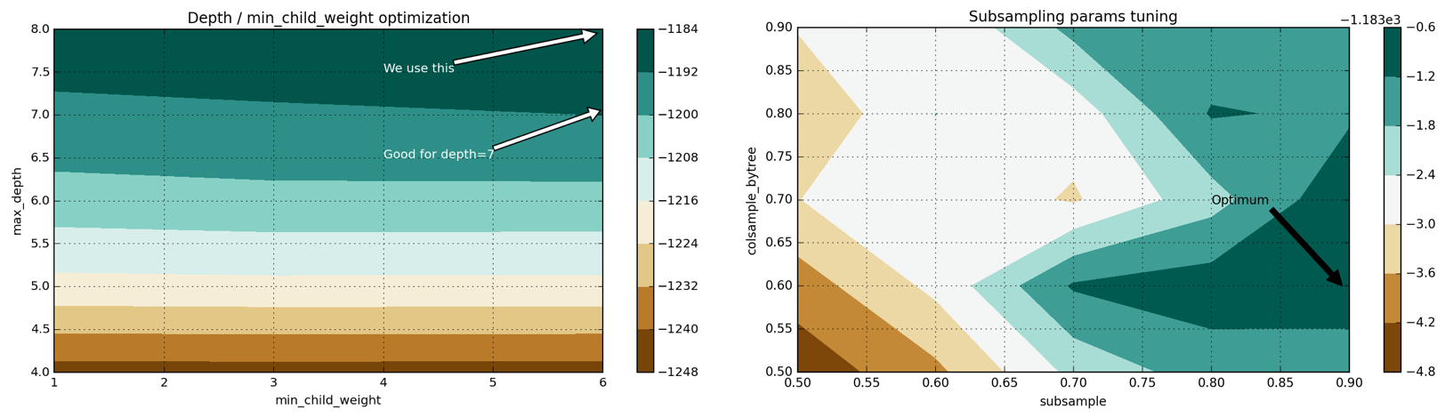
Figure 4: two-dimensional hyperparameter spaces for the max_depth – min_child_weight and colsample-subsampling pairs
Methodology for teaching a multilayer perceptron model:
1.Let's start with a simple one and build a basic model with a single hidden layer (two-layer), the activation function ReLU and the Adam optimizer implementing the gradient descent method. Such shallow models are difficult to retrain, they learn quickly and give good initial results. In terms of a compromise between displacement and dispersion, they are displaced models, but they are stable and give a decent result of MAE = 1190.73 for such a simple model.
2. Use cross-validation with splitting into k parts (k-fold) to measure the performance of deeper models and to visualize retraining. We will train a three-layer model, show that it is easily subject to retraining.
3Add a regularization to the three-layer model: the shutdown of neurons (dropout) and early stopping (early stopping). We define several possible configurations for subsequent manual testing: these configurations differ in the number of hidden elements and the probability of neurons turning off. We will train these models, consider and compare their results obtained by cross-validation, and choose the best one. In fact, with this approach, we will not get any improvements: the results will only worsen compared to the two-layer model. Such an outcome can be caused by a manual (and thus inaccurate) approach to the regularization of the multilayer perceptron. We simply define some reasonable deposition rates for the layers, but there is no guarantee that the selected intensities will be optimal.
four.We will introduce Hyperopt in order to perform a search in the hyper-parameter space in an automated and more intelligent way (we will use tpe.suggest, Parzen estimation algorithms trees). We run several iterations of Hyperopt on numerous hyperparameter configurations with different neuron prolapse, the composition of the layers and the number of hidden elements. Finally, we find out that it is best to use a four-layer architecture (three hidden layers) with the adadelta optimizer, packet normalization (batch normalization), and neuron loss.
The final architecture of the multilayer perceptron:

Figure 5: the final architecture of the multilayer perceptron
The result of this model for cross-validation was: MAE = 1150.009.
Section 2. Learning the first level model
To date, we have trained and configured zero-level models: XGBoost and multilayer perceptron. In this section, we will compile a set of data from zero-level model predictions created during cross-validation (for which true values are known) and test samples of zero-level model predictions that will be used for the final assessment of the metamodel quality.
For a complete acquaintance with the process of building an ensemble of models, please refer to this file.
The ensemble construction methodology that I used is described below:
• Step 1. New training and generation of deferred data set.Since we do not send the results to Kaggle and do not “punch the leaderboard”, we will have to split the training set into two parts: training and test. The training subsample will be used to generate predictions of zero-level models for cross-validation with splitting into k parts (k-fold), whereas the deferred data set will be used only for the final assessment of the performance of the two zero-level models and the metamodel.
• Step 2: Breaking. We divide the training sample into k parts, which will be used to train models of the zero level.
• Step 3: Predictions on cross-validation.Let's train each model of zero level on K-1 parts, we will build predictions for the remaining part. Repeat this process for all K parts. At the end we will get the predictions for the entire test sample (for which we also have tags).
• Step 4: Training throughout the sample. Let's train each of the zero level models on the entire training data set and get the predictions for the test set. Let us compose from the obtained predictions a new data set in which each of the signs is a prediction of one of the zero-level models.
• Step 5: Learning the first level model.We will train the first level model for the predictions obtained by cross-validation, using the corresponding labels from the training sample as labels for the level 1 model. After that, using our combined set of prediction data of the zero level models, we will get the final predictions of the first level model.
We choose linear regression as the first level model: the metamodel is easily subject to retraining (and, frankly, in the competition itself, not much worked better than simple linear regression as a metamodel). This overlay worked very well and significantly improved the results. After cross-validation of zero-level models and the final ensemble model on a hidden data set, we obtained the following results:
The result of the imposition of models MAE = 1136.21 is noticeably better than the result of the best of the models of our ensemble. Of course, this result can be further improved, but in this project we are making a compromise between an increase in the predictive ability of the model and a decrease in training time.
Explanation: This result set was computed on a lazy selection, not through cross-validation. Thus, we have no right to directly compare the results obtained on cross-validation, with the results on the deferred data set. However, a deferred data set is expected to have a distribution close to the distribution of the entire data set. That is why we can argue that the overlap has indeed improved the performance we have achieved.
As a margin note, it would be curious to find out with which weights our zero-level models overlapped. In linear regression, the final prediction is simply a linear combination of weights and initial predictions:
To evaluate our results, we will train and validate our final models (individual and ensemble) on different subsamples of the data set. In this way, we will be able to see how stable our models are and whether they can give a stable result regardless of the initial training sample. To achieve these goals, we will generalize the overlay of models from the Stacking notebook document to the modules / stacker.py class, which allows you to quickly call up the evaluation procedures for our models with different sidami (so that the models are slightly different from each other).
We will train our models of the zero and first levels with 5 different sidami and write the results in a table. Then we use the pd.describe method to get aggregated statistics on the performance of each of the models. The most characteristic metrics here are mean (mean) and standard deviation (std):

As you can see, our models are fairly stable (the standard deviation is low) and the ensemble is always superior to any other model. Its lowest result is better than the best result of the best of the individual models (MAE = 1132.165 versus MAE = 1136.59).
Another explanation: I tried to carefully train and validate models, but there may still be room for information leaks that have gone unnoticed. All models demonstrate improved results, which could be caused by one such leak (but we trained only five models, the parameter seed = 0 could just give the worst results). Nevertheless, the final conclusions remain valid: the averaging of several overlays trained with different sidms improves the final results.
Our basic results are: MAE = 1217.52 (model of a random forest from the company Allstate) and MAE = 1190.73 (MAE of a simple multilayer perceptron). Our final model improved the first result by 7.2% and by 5.1% the second.
To measure the significance of these results, add each of the baseline results to the results table in the previous section, and find out if our baseline results can be called abnormal. So, if the baseline results can be seen as outliers, the difference between our final and baseline results will be significant.
To produce this test, we can calculate the IQR (interquartile range), which is used to detect anomalies and outliers. Then we compute the third data quantile (Q3) and use the formula Q3 + 1.5 * IQR to determine the upper bound of the results. Values above this limit are considered emissions. When conducting this test, we clearly see that both baseline results turn out to be outliers. Thus, we can say that our model overlays far outweigh the base control points.
At the output we get:
Let's abstract from the details and take a look at the project as a whole. We trained and optimized two main models: XGBoost and multilayer perceptron. We have taken a number of steps, from the simplest possible model to the customized, more stable and complex model. After that, we created cross-validation predictions for our level-1 linear regression model, and used the stacking technique to combine the predictions of the zero-level models. Finally, we did a validation of stacking performance and taught him five variations. Averaging the results of these five models, we obtained the final result: MAE = 1129.91.
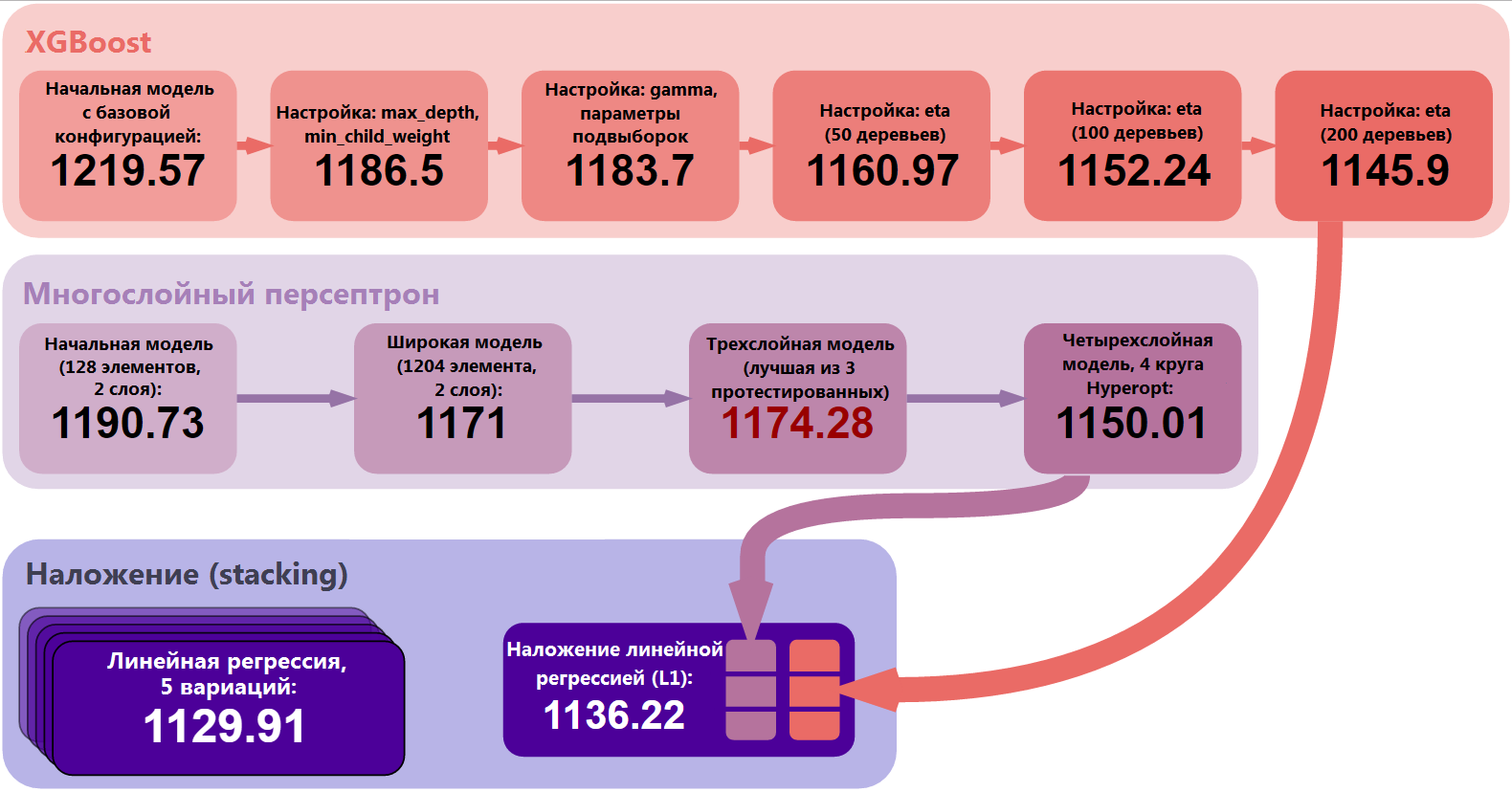
Figure 6: Main stages of improving results
Of course, we could include more models in the zero level, or could make their ensemble more complex. One possible way is to train several completely different ensembles and combine their predictions (for example, as a linear combination) at a new level, level 2.
Complete solution of the problem
The idea of this project was to work with a data set, which does not require the creation of new features. To have such a data set is very nice, because This allows you to focus on algorithms and their optimization, rather than on preprocessing data and making changes to them. Of course, I wanted to experience XGBoost and neural networks in action, and the selected data set could give a good basic assessment of the quality of my model compared to the results of other Kaggle participants.
Even with the weak models given in the project, we obtained a significant excess of the baseline results: by 7.2% . We compared the baseline results with the final results and made sure that the final results are indeed a significant improvement.
Difficulties
This project was not trivial. Although I did not demonstrate any special or creative approaches to the data set, such as creating new features, downgrading or enriching the data, the computational complexity of the models required for Kaggle was higher than I expected.
The main problem in Allstate Claims Severity has become reproducible calculations. To ensure it, a number of prerequisites had to be fulfilled: the process of obtaining the result had to be clear, the calculations — deterministic (or at least with limited oscillations) and reproducible in a reasonable time on any modern equipment. As a result, I greatly reduced the complexity of my existing models and completely eliminated some of the techniques (for example, I excluded the bagging technique for XGBoost and the multi-layer perceptron, although after applying bagging, these models show noticeably better results).
This project was carried out primarily on the Amazon Web Services infrastructure: I used p2.xlarge with GPU computing for a multi-layer perceptron (NVIDIA Tesla K80 GPU, 12 GB of GPU memory) and c4.8xlarge with CPU computing for XGBoost (36 vCPU, 60 GB of memory). There are several sections in my project that require heavy calculations:
• Search by grid. Busting through all the grids in the XGBoost section takes a lot of time. On a regular computer, calculating everything needed for XGBoost can take from one to two hours.
• Cross-validation of multi-layer perceptron models. Unfortunately, there is no magic way to accelerate cross-validation in training a multi-layer perceptron. To assess the quality of the model, cross-validation is a reliable method, it should not be avoided, but it should be enough time.
• Optimization of hyperparameters. This is definitely the hardest part of all the calculations. Looking through various combinations of hyperparameters and finding the right one with Hyperopt takes many hours.
• Generate cross-validation predictions for the multilayer perceptron and XGBoost.
The best way to reproduce my results would be to first run the pre-trained models and then recalculate some of the easiest of them.
The project leaves ample space for future improvements. Below, I reflect on what other improvements can be used.
Preliminary data processing
1. I first started working on a model of a multi-layer perceptron, and only then discovered a technique with logarithm of the target variable. As a result, my multilayer perceptrons were trained without a logarithmic transformation. Of course, it is possible and necessary to log the target variable and re-train all models of the multilayer perceptron.
2. A promising way to transform the target variable would be to move it 200 points to the right (add 200 to all values). If we make such a shift and then take the logarithm, we will get rid of the outliers on the left side of the distribution density function of the target variable. Thus, we will make its distribution closer to normal.
Xgboost
1. Train a more sophisticated XGBoost model, adding more trees and at the same time reducing the eta parameter. My working model uses 28 thousand trees and eta = 0.003, which was determined using the grid search procedure.
2. Use early_stopping_rounds instead of num_boost_round to stop learning and avoid retraining the model. In this case, set eta a small number and num_boost_round very large (up to 100 thousand). We need to understand that in this case we will have to prepare a validation sample. As a result, our model will receive less data for training, and its performance may fall.
3. Run the grid search procedure at other hyperparameter values. Let's say you could test the colsample_bytree values between 0 and 0.5, which often bring good results. The idea here is that there are several local optima in the hyper-parameter space and we should find several of them.
4. Combine several XGBoost models trained with different hyperparameter values. We can make such a union by averaging the results of the models, blending (blending) and imposing (stacking).
Multilayer perceptron
1. Use the bagging technique to averaging several multilayer perceptrons of the same model. Our model is stochastic (for example, because we use neuronal loss = dropout), therefore bagging will smooth its work and improve predictive ability.
2. Try a deeper network architecture, other element configurations, and hyperparameter values. You can test other optimizers using the gradient descent method, change the number of layers, the number of elements in each layer - all the power of Hyperopt is in our hands.
3. Combine several different multilayer perceptrons (for example, train a two-layer, three-layer and four-layer neural network), using any of the techniques you know. These models will cover the data space in different ways and provide improvements over the baseline results.
Cross validation
Instead of using simple cross-validation with splitting into 3 parts (sometimes we used splitting into 5 parts), we can proceed to cross-validation into 10 parts. Such cross-validation is more suitable for Kaggle competitions, but will almost certainly improve our results (we will have more training data).
Stacking
1. You can add more zero-level models to the ensemble. First, we can simply train more multilayer perceptrons and XGBoost models, but they should be different from each other. For example, we can train these models on different subsets of data, for some of them we can pre-process data in different ways (loss). Secondly, we can introduce completely other models: LightGBM, algorithm of k nearest neighbors, factorization machines (FM), etc.
2. Another idea is to add the second level as a new overlay layer. As a result, we get a two-level stacking: we still have zero-level regressors (L0), out-of-fold predictions of which we teach several different first-level metamodels (L1). Then, we simply take a linear combination of the predictions of the metamodel (L2) - and we get the final estimate.
3. Try to use PCA - the principal component method, which was reviewed in a laptop about data research. There are a few ideas here. First, the resulting components can be mixed into out-of-fold predictions that linear regression (L1) will be trained in to add additional information to the metamodel. Secondly, it is possible to select from all the signs only those that have a high weight, and discard the rest as noise. Sometimes it also helps to improve the quality of the resulting model.
Description of the configuration on which the entire project was executed, here
Report on the diploma project "Prediction of the severity of insurance requirements for the company Allstate"
Part 1. Project Description
General project overview
Many people working in data-related areas have heard of Kaggle, the platform for data science competitions. Today, more than 600 thousand data scientists and many well-known companies are represented at Kaggle. The company describes its problem, sets quality metrics, publishes a set of data that could help solve it, and participants find original ways to solve the problem posed by the company.
This Kaggle competition is sponsored by Allstate, the largest publicly traded company in the United States in the personal and life insurance business. At the moment, Allstate is developing automatic methods for predicting the cost (severity) of insurance claims and has asked the Kaggle community to demonstrate fresh ideas and new approaches to solving this problem.
The company seeks to improve the quality of its services in processing insurance claims and has published a set of data on accidents that have occurred in households (each household is represented by an anonymized feature vector) with a numerical estimate of the value of the insurance claim. Our task was to predict the severity of a possible insurance claim for a new household.
')
Several more data sets related to this task are also available on Kaggle:
• Allstate insurance claims prediction competition - an earlier Allstate competition, the purpose of which was to predict insurance premiums based on the characteristics of the insured vehicle. The data set of this competition provides an opportunity to dive into the insurance field.
• The fire loss assessment competition is a competition held by the Liberty Mutual Group and aimed at predicting the expected fire losses to form the terms of insurance contracts. This is another example of a data set from the insurance industry that helped us gain an understanding of the approaches to solving prediction problems in the insurance industry.
Separately, I note that the original data set is highly anonymous (both in terms of the names of features and in terms of values). This aspect complicates both the understanding of the meaning of the signs and the enrichment of the data set from external sources. Competitors tried differently to enrich and interpret the original data, but the success of their attempts remains controversial. On the other hand, there seems to be no data leakage in this data set, which occurs when additional information remains in the training data. Such information can be highly correlated with the target variable and lead to unreasonably accurate predictions. Recently, a large number of Kaggle competitions have suffered from such leaks.
Formulation of the problem
We have at our disposal a data set containing records for the insurance claims of Allstate’s customers. Each entry contains both categorical and continuous signs. The target variable is a numerical estimate of the losses caused by this insurance claim. All signs are made as anonymous as possible: we do not know either the real names of the signs or their true meanings.
Our goal is to build a model that will be able to predict future losses correctly on the basis of given values of attributes. Obviously, this is a regression task: target variable is numerical. This is also the task of teaching with the teacher: the target variable is clearly defined in the training data set, and we need to get its values for each record of the test set.
Allstate did a great job of cleaning and preprocessing the data: the data set provided is very clean and (after some additional processing) can be transferred to a large number of learning algorithms with the teacher. As we will see in the part of the data research report, the task of Allstate does not specifically allow generating new features or preprocessing existing features. On the other hand, this datasset pushes the use and testing of various machine learning algorithms and ensembles - just what is needed for a graduation project.
I applied the following approach to the Allstate project:
1. Investigate the data set, understand the meaning of the data, the characteristics and the target variable, and find simple relationships in the data. This step is performed in the Data Discovery notebook file .
2. Perform the necessary data preprocessing and train several different machine learning algorithms (XGBoost and multilayer perceptron). Get baseline results. These tasks are solved in the XGBoost and MLP files.
3. Adjust the models and achieve a noticeable improvement in the results for each of them. This step is also implemented in the XGBoost and MLP files.
4. Train the ensemble using the overlaying technique of models (stacking) using the previous models as basic predictors. Get the final results that will be significantly better than the previous ones. This stage is implemented in the Stacking notebook file.
5. Briefly discuss the results, assess the final position in the tournament standings and find additional ways to improve it. We’ll talk about the results below in this report and in the last part of the Stacking notebook file.
Metrics
The Kaggle platform requires the company conducting the competition to clearly define the metrics on which participants can compete. Allstate chose MAE as such a metric. MAE (mean absolute error) is a very simple and obvious metric that directly compares the predicted and true values.
This metric is set and cannot be changed, because is part of the competition conditions. Nevertheless, I consider it well suited to this task. Firstly, MAE (as opposed to MSE or RMS error) does not give a large penalty for an incorrect estimate of emissions (there are several emissions with abnormally high loss values in the data sheet). Secondly, MAE is easy to understand: error values are expressed in the same dimensions as the target variable itself. Generally speaking, MAE is a good metric for beginners in data science. It is easy to compute, easy to understand, and difficult to misinterpret.
Part 2. Analysis
Examine the data
For a complete acquaintance with this stage, you can refer to the Data Discovery file.
The entire training sample consists of 188318 elements indexed by the variable uid. The index for working with data does not carry additional information, since it's just a numbering, starting with “1” with some missing values. We are not going to use a test set without an index for prediction (it is necessary to send results to Kaggle), however it is worth noting that the test data set is organized in the same way as the training set. Obviously, the training and test samples were obtained from one data set by a partitioning procedure, for example, train_test_split from the sklearn package.
The main results of this part of the project are as follows:
• The data set contains 130 different signs (without taking into account the id index and the target loss variable). Given the size of the data set, this is quite a reasonable number of signs. We could hardly face the "curse of dimension" here.
• 116 signs categorical, 14 numerical. We will probably need to encode these 116 features, since most machine learning algorithms cannot correctly handle categorical variables. We will discuss the ways of such coding and the differences between them later.
• There are no missing values in the entire data set. This fact only confirms that Allstate provided data with a high degree of preprocessing in order to make it accessible and easy to use.
• Most categorical features (72 or 62%) are binary (yes / no; male / female), but their meanings are written simply as “A” and “B”, so we cannot guess their meaning at all. 3 signs take three different values, 12 signs - 4 different values.
• Numerical signs are already scaled in the range from 0 to 1, standard deviations for all of them are close to 0.2, average values are about 0.5, therefore we cannot make any assumptions about their values for these signs.
• Apparently, some numerical traits used to be categorical before they were converted to numerical traits using LabelEncoder or a similar procedure.
• By constructing histograms of various signs, you can make sure that none of them obeys the normal distribution law. You can try to reduce the asymmetry of the distribution of these data (in the case of scipy.stats.mstats.skew> 0.25), but even after such a conversion, it will not be possible to achieve a distribution that is close to normal.
• The target variable is also not normally distributed, although it can be reduced to a normal distribution by a simple logarithmic transformation.
• The target variable contains several outliers with abnormally high values (very serious incidents). Ideally, we would like our model to be able to identify and correctly predict such outliers. At the same time, we can easily retrain them if we are not careful enough. It is clear that some compromise is needed here.
• The training and test samples have similar data distributions. This is an ideal breakdown characteristic for training and test samples, which greatly simplifies cross-validation and allows us to make informed decisions about the quality of models using cross-validation in the training data set. This greatly simplified participation in the Kaggle competition, but it would not be useful to complete the graduation project.
• Several continuous features are highly correlated (the correlation matrix is shown in Fig. 1 below). This leads to data-based multicollinearity in this data set, which can drastically reduce the predictive ability of linear regression models. Part of this problem can be solved with L1 or L2 regularization.
Figure 1: Correlation matrix for continuous features
Survey Visualization
I will show one visualization in order to demonstrate an important feature of this data set - a high degree of anonymity, preprocessing of data.
Below are histograms of 14 continuous signs labeled as cont #. As can be seen from fig. 1, the data distributions may have multiple peaks, and the density functions of the distributions are not close to Gaussian. We could try to reduce the data asymmetry factor, but the use of normalization algorithms (for example, the Box-Cox transform) did little for this data set.
Figure 2: Continuous features histograms
The cont2 feature is especially interesting. This feature was apparently derived from the categorical and may reflect the age or age category. Unfortunately, I did not go deep into the study of this feature: he had no influence on my project.
Algorithms and methods of data analysis
This section is much more detailed in the following two documents: XGBoost notebook and MLP notebook .
XGBoost. One of the reasons for my interest in the project is the opportunity to try the method of boosting over trees and, in particular, XGBoost. De facto, this algorithm has become a kind of standard Swiss knife for many Kaggle competitions due to its scalability, flexibility and impressive predictive power.
XGBoost is suitable for teacher learning tasks similar to the one we have (clearly defined training data set and target variable). Below we describe the principles of the XGBoost algorithm.
XGBoost, in essence, is a variation of boosting — an ensemble meta-algorithm for machine learning, used to reduce bias and variance in teacher training, and a family of machine learning algorithms that turn weaker models into stronger ones. Source: Wikipedia . Initially, the ideas of boosting are rooted in the question posed by Kearns and Valiant, whether “weak” learning algorithms that give results a little better than random guessing in a PAC (probably approximately correct) model, can be “strengthened” to a “strong” learning algorithm arbitrary accuracy. Source: A brief introduction to boosting (Yoav Freund and Robert E. Schapire). An affirmative answer to this question was given to RESchapire in his article The Strength of Weak Learning , which led to the development of many boosting algorithms.
As you can see, the fundamental principle of boosting is the consistent application of weak learning algorithms. Each successive weak algorithm attempts to reduce the displacement of the entire model, thus combining weak algorithms into a powerful ensemble model. Many different examples of algorithms and methods of boosting can be given, such as AdaBoost (adaptive boosting, which adapts to weak learning algorithms), LPBoost and gradient boosting.
XGBoost, in particular, is a library that implements a gradient boosting scheme. Gradient boosting models are built in stages, just as with other boosting methods. This boosting method generalizes weak learning algorithms, allowing optimization of an arbitrary differentiable loss function (loss function with a computable gradient).
XGBoost, as a kind of boosting, includes an original decision tree-based machine learning algorithm suitable for working with sparse data; theoretically sound procedure allows you to work with weights of various elements in the training of trees. Source: XGBoost: scalable tree-boosting system (Tianqi Chen, Carlos Guestrin)
There are several advantages of the XGBoost algorithm:
• Regularization. As will be shown in the section on the model of a multilayer perceptron, using other algorithms one can easily obtain a retrained model. XGBoost provides very reliable ready-to-use regularization tools along with a set of parameters to customize this process. The list of these parameters includes: gamma (the minimum reduction of the loss function required for further tree division), alpha (weight for L1 regularization), lambda (weight for L2 regularization), max_depth (maximum depth of the tree), min_child_weight (minimum sum of all weights observations required for the child).
• Implementation of parallel and distributed computing. Unlike many other boosting algorithms, training here can be done in parallel, thereby reducing training time. XGBoost works really fast. According to the authors of the aforementioned article, “the system works more than 10 times faster than existing popular solutions already on one computer and can be scaled to millions of copies in a distributed or memory-limited environment.”
• Integrated cross-validation. Cross-validation is a prerequisite for assessing the quality of the resulting model, and in the case of XGBoost, its process of working with it is extremely simple and straightforward.
MLP. The second model we are building is a fully connected direct propagation neural network or a multilayer perceptron. Since our ultimate goal is to build an ensemble (stacking) of basic regressors (and we decided on the type of the first one, XGBoost), we need to find another “type” of a generalizing algorithm that will otherwise examine our data set.
This is when they mean when they say that generalizing algorithms of level zero should “cover space”. Wolpert, Generalization overlay.
By adding more layers and more elements within each layer, the neural network can capture very complex non-linear connections in the data. The universal approximation theorem states that a direct propagation neural network can approximate any continuous function in Euclidean space. Thus, the multilayer perceptron is a very powerful simulation algorithm. Multilayer perceptrons are easily subject to retraining, but we have all the necessary tools at our disposal to reduce the influence of this factor: accidental deactivation of neuron activation (dropout), L1-L2 regularization, packet normalization (batch normalization), etc. We can also train several similar neural networks and average their predictions.
The deep learning community has developed high-quality software for learning and evaluating models based on artificial neural networks. My models are based on TensorFlow , a library for tensor computing developed by Google. To simplify the construction of models, I decided to use Keras , a high-level front end for TensorFlow and Theano, which takes over most of the standard operations needed to build and train neural networks.
GridSearch and Hyperopt. These methods are used to select models and configure hyperparameters. While the GridSearch (grid search) exhaustively enumerates all possible combinations of parameters, Hyperopt either selects a given number of candidates from the parameter space with a given distribution, or uses a form of Bayesian optimization. Together with both of these selection methods, we use a cross-validation technique to assess model performance. We use cross-validation with splitting into k parts (k-fold) with three or five parts depending on the computational complexity of the model.
Overlay models (stacking). We combine the predictions of two of our models (XGBoost and the multilayer perceptron) to construct the final prediction using a meta-regressor. This method is called stacking and is used extensively on Kaggle (often excessively). The idea of stacking is to split the training sample into k parts and train each of the basic regressors into k-1 parts, making predictions for the rest. As a result, we get a training sample with regressor predictions (out-of-fold), while having real values of the target variable. Next, we train the metamodel on this data, using the predictions of each regressor as a sign for the metamodel, and the true values as the target sign.
To the trained metamodel, we input the regressor prediction for the test sample and we get the final predictions in which the trained model takes into account the characteristic errors of each regressor. The implementation of this stage is described in detail in the Stacking notebook file .
Criteria for evaluating results
The first result was given by Allstate: they trained an ensemble model of a random forest and got the result MAE = 1217.52141. This result is easily surpassed even by a simple XGBoost model, and most of the participants succeeded.
I also set several criteria for myself when I was teaching models. The bottom line for me was the performance of a simple model of this class. For XGBoost, this result was set to MAE = 1219.57, it is achieved by a simple model of 50 trees without any optimization or adjustment of the hyperparameters. I took the standard values of the hyperparameters (suggested in the article from Analytics Vidhya ), left a small number of trees and got this starting result.
For a multilayer perceptron, the performance of a two-layer model with a small number of elements in its hidden layer (128) with the ReLU activation function, standard initialization of weights and the Adam GD optimizer: MAE = 1190.73 was chosen as the baseline result.
In this thesis project, I avoided complex baseline-models, because I understand that all the results should be reproducible. I also participate in this Kaggle competition, but learning all my models used in the competition, most of which are combinations and uses a large number of algorithms, will definitely require too much time from the reader. In the Kaggle competition, I hope to surpass the result of MAE = 1100.
Part 3. Methodology
Preliminary data processing
I already mentioned that this dataset was already well prepared and pre-processed, for example, continuous attributes were scaled to the interval [0,1], categorical attributes were renamed, their values were turned into numbers. In fact, in terms of preprocessing, there is not much left that could be done. However, some work still needs to be done in order to train the correct models.
Target variable pre-processing
Our target attribute has an exponential distribution, which can lower the quality of regression models. As you know, regression models work best when the target variable is distributed normally.
To solve this problem, we simply apply a logarithmic transformation to the target variable loss: np.log (train ['loss']).
Figure 3: Histograms of the distribution of the target variable before and after the logarithmic transformation
The result can be improved: to the left of the main distribution bell several deviating observations lie. To get rid of these emissions, we can shift all the values of the loss variable by 200 points to the right (loss + 200) and then take the logarithm from them.
Coding categorical variables
Most machine learning algorithms cannot directly work with categorical variables. XGBoost is no exception here, so we will need to convert our categorical variables to numeric ones. Here we can choose one of two standard strategies: label coding (label encoding) or direct coding (one-hot encoding). What strategy to use is a rather controversial question, but here several factors should be considered:
Directly encoding (one-hot encoding) is the basic way of working with categorical features. It produces a sparse matrix, where each new column represents one possible value of a single feature. Since we have 116 categorical variables, and the variable cat116 takes 326 values, we can get a sparse matrix with a huge number of zeros. This will lead to longer training, increase memory costs and may even worsen the final results. Another disadvantage of direct coding is the loss of information in cases where the order of categories is important.
Label encoding , on the other hand, simply normalizes the input data column so that it contains only values between 0 and the number of classes -1. For many regression algorithms, this is not a very good strategy, but XGBoost can cope and does this transformation very well.
For XGBoost we will use LabelEncoder and normalize the input data. For a multilayer perceptron, we will need to create dummy variables, so our choice here is one-hot encoding.
Implementation and improvement of models
As mentioned earlier, our methodology for implementing machine learning will be divided into two sections:
• Training, tuning, and cross-validation of base models (zero-level models): XGBoost and multilayer perceptron, assuming that we have already made preliminary data preparation, which is slightly different for these two models. The difference will be in the coding of the signs (direct or coding of the tags) and (unfortunately) in the absence of a logarithmic transformation of the target variable for the multilayer perceptron model. The result of this part will be two customized models, the results of which will meet the established criteria.
• Training and validation of a level 1 model, that is, overlay models. The result of this section will be a new metamodel, giving better results than each of the basic zero-level models that we have previously taught.
Now it's time to give a detailed overview of each section.
Section 1. Zero-level models: training, tuning, cross-validation.
The XGBoost model learning methodology (adapted from the Analytics Vidhya XGBoost customization tutorial ):
1. Teach the shallow and simple model with the parameters num_boost_round = 50, max_depth = 5 and get the basic result MAE = 1219.57. We will set this result as a lower bound and will improve it by adjusting the model.
2To facilitate the optimization of hyperparameters, we implement our own class XGBoostRegressor, built on XGBoost. Such a class, by and large, is not necessary for the model to work, however, it will give us a number of advantages (we can use our own loss function and minimize this function instead of maximizing) when using the GridSearchCV grid search implemented in scikit-learn.
3. We will determine and fix the learning rate and the number of trees that will be in each subsequent iteration over the grid. Since our task is to get a good result in the minimum time, we will put a small number of trees and a high learning rate: eta = 0.1, num_boost_round = 50.
four.Set the max_depth and min_child_weight parameters. These hyperparameters are recommended to be configured together, since increasing max_depth increases the complexity of the model (and increases the likelihood of retraining). At the same time, min_child_weight acts as a regularizing parameter. We get the following best parameters: max_depth = 8, min_child_weight = 6. This improves the results from MAE = 1219.57 to MAE = 1186.5.
5. Configure gamma, the regularization parameter.
6. Set the ratio of the number of features and training elements that will be used in each of the trees: colsample_bytree, subsample. We get the following optimal configuration: subsample = 0.9, colsample_bytree = 0.6 and improve our results to MAE = 1183.7.
7Finally, add more trees (increase the parameter num_boost_round) and reduce the intensity of learning eta. We will also develop a rule of thumb for understanding the relationship between these two hyperparameters. Our final model uses 200 trees, has eta = 0.07 and the final result is MAE = 1145.9.
An example of the process of setting up model parameters using Grid Search is shown in Figure 4 below (for details, see this file):
Figure 4: two-dimensional hyperparameter spaces for the max_depth – min_child_weight and colsample-subsampling pairs
Methodology for teaching a multilayer perceptron model:
1.Let's start with a simple one and build a basic model with a single hidden layer (two-layer), the activation function ReLU and the Adam optimizer implementing the gradient descent method. Such shallow models are difficult to retrain, they learn quickly and give good initial results. In terms of a compromise between displacement and dispersion, they are displaced models, but they are stable and give a decent result of MAE = 1190.73 for such a simple model.
2. Use cross-validation with splitting into k parts (k-fold) to measure the performance of deeper models and to visualize retraining. We will train a three-layer model, show that it is easily subject to retraining.
3Add a regularization to the three-layer model: the shutdown of neurons (dropout) and early stopping (early stopping). We define several possible configurations for subsequent manual testing: these configurations differ in the number of hidden elements and the probability of neurons turning off. We will train these models, consider and compare their results obtained by cross-validation, and choose the best one. In fact, with this approach, we will not get any improvements: the results will only worsen compared to the two-layer model. Such an outcome can be caused by a manual (and thus inaccurate) approach to the regularization of the multilayer perceptron. We simply define some reasonable deposition rates for the layers, but there is no guarantee that the selected intensities will be optimal.
four.We will introduce Hyperopt in order to perform a search in the hyper-parameter space in an automated and more intelligent way (we will use tpe.suggest, Parzen estimation algorithms trees). We run several iterations of Hyperopt on numerous hyperparameter configurations with different neuron prolapse, the composition of the layers and the number of hidden elements. Finally, we find out that it is best to use a four-layer architecture (three hidden layers) with the adadelta optimizer, packet normalization (batch normalization), and neuron loss.
The final architecture of the multilayer perceptron:
Figure 5: the final architecture of the multilayer perceptron
The result of this model for cross-validation was: MAE = 1150.009.
Section 2. Learning the first level model
To date, we have trained and configured zero-level models: XGBoost and multilayer perceptron. In this section, we will compile a set of data from zero-level model predictions created during cross-validation (for which true values are known) and test samples of zero-level model predictions that will be used for the final assessment of the metamodel quality.
For a complete acquaintance with the process of building an ensemble of models, please refer to this file.
The ensemble construction methodology that I used is described below:
• Step 1. New training and generation of deferred data set.Since we do not send the results to Kaggle and do not “punch the leaderboard”, we will have to split the training set into two parts: training and test. The training subsample will be used to generate predictions of zero-level models for cross-validation with splitting into k parts (k-fold), whereas the deferred data set will be used only for the final assessment of the performance of the two zero-level models and the metamodel.
• Step 2: Breaking. We divide the training sample into k parts, which will be used to train models of the zero level.
• Step 3: Predictions on cross-validation.Let's train each model of zero level on K-1 parts, we will build predictions for the remaining part. Repeat this process for all K parts. At the end we will get the predictions for the entire test sample (for which we also have tags).
• Step 4: Training throughout the sample. Let's train each of the zero level models on the entire training data set and get the predictions for the test set. Let us compose from the obtained predictions a new data set in which each of the signs is a prediction of one of the zero-level models.
• Step 5: Learning the first level model.We will train the first level model for the predictions obtained by cross-validation, using the corresponding labels from the training sample as labels for the level 1 model. After that, using our combined set of prediction data of the zero level models, we will get the final predictions of the first level model.
We choose linear regression as the first level model: the metamodel is easily subject to retraining (and, frankly, in the competition itself, not much worked better than simple linear regression as a metamodel). This overlay worked very well and significantly improved the results. After cross-validation of zero-level models and the final ensemble model on a hidden data set, we obtained the following results:
MAE XGBoost: 1149.19888471 MAE : 1145.49726607 MAE : 1136.21813333 The result of the imposition of models MAE = 1136.21 is noticeably better than the result of the best of the models of our ensemble. Of course, this result can be further improved, but in this project we are making a compromise between an increase in the predictive ability of the model and a decrease in training time.
Explanation: This result set was computed on a lazy selection, not through cross-validation. Thus, we have no right to directly compare the results obtained on cross-validation, with the results on the deferred data set. However, a deferred data set is expected to have a distribution close to the distribution of the entire data set. That is why we can argue that the overlap has indeed improved the performance we have achieved.
As a margin note, it would be curious to find out with which weights our zero-level models overlapped. In linear regression, the final prediction is simply a linear combination of weights and initial predictions:
PREDICTION = 0.59 * XGB_PREDICTION + 0.41 * MLP_PREDICTION Part 4. Results
Model Evaluation and Validation
To evaluate our results, we will train and validate our final models (individual and ensemble) on different subsamples of the data set. In this way, we will be able to see how stable our models are and whether they can give a stable result regardless of the initial training sample. To achieve these goals, we will generalize the overlay of models from the Stacking notebook document to the modules / stacker.py class, which allows you to quickly call up the evaluation procedures for our models with different sidami (so that the models are slightly different from each other).
We will train our models of the zero and first levels with 5 different sidami and write the results in a table. Then we use the pd.describe method to get aggregated statistics on the performance of each of the models. The most characteristic metrics here are mean (mean) and standard deviation (std):
As you can see, our models are fairly stable (the standard deviation is low) and the ensemble is always superior to any other model. Its lowest result is better than the best result of the best of the individual models (MAE = 1132.165 versus MAE = 1136.59).
Another explanation: I tried to carefully train and validate models, but there may still be room for information leaks that have gone unnoticed. All models demonstrate improved results, which could be caused by one such leak (but we trained only five models, the parameter seed = 0 could just give the worst results). Nevertheless, the final conclusions remain valid: the averaging of several overlays trained with different sidms improves the final results.
Justification
Our basic results are: MAE = 1217.52 (model of a random forest from the company Allstate) and MAE = 1190.73 (MAE of a simple multilayer perceptron). Our final model improved the first result by 7.2% and by 5.1% the second.
To measure the significance of these results, add each of the baseline results to the results table in the previous section, and find out if our baseline results can be called abnormal. So, if the baseline results can be seen as outliers, the difference between our final and baseline results will be significant.
To produce this test, we can calculate the IQR (interquartile range), which is used to detect anomalies and outliers. Then we compute the third data quantile (Q3) and use the formula Q3 + 1.5 * IQR to determine the upper bound of the results. Values above this limit are considered emissions. When conducting this test, we clearly see that both baseline results turn out to be outliers. Thus, we can say that our model overlays far outweigh the base control points.
for baseline in [1217.52, 1190.73]: stacker_scores = list(scores.stacker) stacker_scores.append(baseline) max_margin = np.percentile(stacker_scores, 75) + 1.5*iqr(stacker_scores) if baseline - max_margin > 0: print 'MAE =', baseline, ' .' else: print 'MAE = ', baseline, ' .' At the output we get:
MAE = 1217.52 . MAE = 1190.73 . Part 5. Conclusion
Free form visualization
Let's abstract from the details and take a look at the project as a whole. We trained and optimized two main models: XGBoost and multilayer perceptron. We have taken a number of steps, from the simplest possible model to the customized, more stable and complex model. After that, we created cross-validation predictions for our level-1 linear regression model, and used the stacking technique to combine the predictions of the zero-level models. Finally, we did a validation of stacking performance and taught him five variations. Averaging the results of these five models, we obtained the final result: MAE = 1129.91.
Figure 6: Main stages of improving results
Of course, we could include more models in the zero level, or could make their ensemble more complex. One possible way is to train several completely different ensembles and combine their predictions (for example, as a linear combination) at a new level, level 2.
Analysis of the work done
Complete solution of the problem
The idea of this project was to work with a data set, which does not require the creation of new features. To have such a data set is very nice, because This allows you to focus on algorithms and their optimization, rather than on preprocessing data and making changes to them. Of course, I wanted to experience XGBoost and neural networks in action, and the selected data set could give a good basic assessment of the quality of my model compared to the results of other Kaggle participants.
Even with the weak models given in the project, we obtained a significant excess of the baseline results: by 7.2% . We compared the baseline results with the final results and made sure that the final results are indeed a significant improvement.
Difficulties
This project was not trivial. Although I did not demonstrate any special or creative approaches to the data set, such as creating new features, downgrading or enriching the data, the computational complexity of the models required for Kaggle was higher than I expected.
The main problem in Allstate Claims Severity has become reproducible calculations. To ensure it, a number of prerequisites had to be fulfilled: the process of obtaining the result had to be clear, the calculations — deterministic (or at least with limited oscillations) and reproducible in a reasonable time on any modern equipment. As a result, I greatly reduced the complexity of my existing models and completely eliminated some of the techniques (for example, I excluded the bagging technique for XGBoost and the multi-layer perceptron, although after applying bagging, these models show noticeably better results).
This project was carried out primarily on the Amazon Web Services infrastructure: I used p2.xlarge with GPU computing for a multi-layer perceptron (NVIDIA Tesla K80 GPU, 12 GB of GPU memory) and c4.8xlarge with CPU computing for XGBoost (36 vCPU, 60 GB of memory). There are several sections in my project that require heavy calculations:
• Search by grid. Busting through all the grids in the XGBoost section takes a lot of time. On a regular computer, calculating everything needed for XGBoost can take from one to two hours.
• Cross-validation of multi-layer perceptron models. Unfortunately, there is no magic way to accelerate cross-validation in training a multi-layer perceptron. To assess the quality of the model, cross-validation is a reliable method, it should not be avoided, but it should be enough time.
• Optimization of hyperparameters. This is definitely the hardest part of all the calculations. Looking through various combinations of hyperparameters and finding the right one with Hyperopt takes many hours.
• Generate cross-validation predictions for the multilayer perceptron and XGBoost.
The best way to reproduce my results would be to first run the pre-trained models and then recalculate some of the easiest of them.
Improvements
The project leaves ample space for future improvements. Below, I reflect on what other improvements can be used.
Preliminary data processing
1. I first started working on a model of a multi-layer perceptron, and only then discovered a technique with logarithm of the target variable. As a result, my multilayer perceptrons were trained without a logarithmic transformation. Of course, it is possible and necessary to log the target variable and re-train all models of the multilayer perceptron.
2. A promising way to transform the target variable would be to move it 200 points to the right (add 200 to all values). If we make such a shift and then take the logarithm, we will get rid of the outliers on the left side of the distribution density function of the target variable. Thus, we will make its distribution closer to normal.
Xgboost
1. Train a more sophisticated XGBoost model, adding more trees and at the same time reducing the eta parameter. My working model uses 28 thousand trees and eta = 0.003, which was determined using the grid search procedure.
2. Use early_stopping_rounds instead of num_boost_round to stop learning and avoid retraining the model. In this case, set eta a small number and num_boost_round very large (up to 100 thousand). We need to understand that in this case we will have to prepare a validation sample. As a result, our model will receive less data for training, and its performance may fall.
3. Run the grid search procedure at other hyperparameter values. Let's say you could test the colsample_bytree values between 0 and 0.5, which often bring good results. The idea here is that there are several local optima in the hyper-parameter space and we should find several of them.
4. Combine several XGBoost models trained with different hyperparameter values. We can make such a union by averaging the results of the models, blending (blending) and imposing (stacking).
Multilayer perceptron
1. Use the bagging technique to averaging several multilayer perceptrons of the same model. Our model is stochastic (for example, because we use neuronal loss = dropout), therefore bagging will smooth its work and improve predictive ability.
2. Try a deeper network architecture, other element configurations, and hyperparameter values. You can test other optimizers using the gradient descent method, change the number of layers, the number of elements in each layer - all the power of Hyperopt is in our hands.
3. Combine several different multilayer perceptrons (for example, train a two-layer, three-layer and four-layer neural network), using any of the techniques you know. These models will cover the data space in different ways and provide improvements over the baseline results.
Cross validation
Instead of using simple cross-validation with splitting into 3 parts (sometimes we used splitting into 5 parts), we can proceed to cross-validation into 10 parts. Such cross-validation is more suitable for Kaggle competitions, but will almost certainly improve our results (we will have more training data).
Stacking
1. You can add more zero-level models to the ensemble. First, we can simply train more multilayer perceptrons and XGBoost models, but they should be different from each other. For example, we can train these models on different subsets of data, for some of them we can pre-process data in different ways (loss). Secondly, we can introduce completely other models: LightGBM, algorithm of k nearest neighbors, factorization machines (FM), etc.
2. Another idea is to add the second level as a new overlay layer. As a result, we get a two-level stacking: we still have zero-level regressors (L0), out-of-fold predictions of which we teach several different first-level metamodels (L1). Then, we simply take a linear combination of the predictions of the metamodel (L2) - and we get the final estimate.
3. Try to use PCA - the principal component method, which was reviewed in a laptop about data research. There are a few ideas here. First, the resulting components can be mixed into out-of-fold predictions that linear regression (L1) will be trained in to add additional information to the metamodel. Secondly, it is possible to select from all the signs only those that have a high weight, and discard the rest as noise. Sometimes it also helps to improve the quality of the resulting model.
Description of the configuration on which the entire project was executed, here
Source: https://habr.com/ru/post/317246/
All Articles