Limit the speed of traffic. Policer or shaper, what to use on the net?

When it comes to limiting bandwidth on network equipment, two technologists first come to mind: policer and shaper. Policer limits the speed by discarding "extra" packets that lead to the excess of a given speed. Shaper tries to smooth the speed to the desired value by buffering the packets. I decided to write this article after reading notes on the blog of Ivan Pepelnyak (Ivan Pepelnjak). It once again raised the question: what is better - a policer or a shaper. And as often happens with such questions, the answer is: it all depends on the situation, since each of the technologies has its pros and cons. I decided to deal with this a little more, by carrying out some simple experiments. The results are rolled up.
And so, let's start with a general picture of the difference between a policer and a shaper.
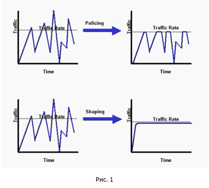
As you can see, the policer cuts off all the peaks, shaper does smoothing our traffic. A pretty good comparison between the policer and the shaper can be found here .
')
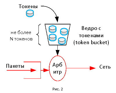
Both technologies basically use the token mechanism. In this mechanism, there is a virtual bucket limited in size (token bucket), into which tokens flow with some regularity. Token, as a travel card, is consumed for the transfer of packets. If there are no tokens in the bucket, then the packet is discarded (other actions can be performed). Thus, we get a constant traffic transfer rate, since the tokens go to the bucket in accordance with the given speed.
Maybe it was worth making it easier?
The session speed is usually measured in the allotted time interval, for example, in 5 seconds or 5 minutes. Taking an instantaneous value is meaningless, since data is always transmitted at the speed of the channel. Moreover, if we do the averaging over different time intervals, we will get different graphs of the data transfer rate, since the traffic in the network is not uniform. I think anyone came across this by building graphs in the monitoring system.
The mechanism of tokens allows for flexibility in setting the speed limit. The size of the bucket affects how we average our speed. If the bucket is large (i.e., there can be a lot of tokens there), we will allow traffic to “jump out” more than the allotted limits at certain points in time (equivalent to averaging over a longer period of time). If the bucket size is small, the traffic will be more uniform, rarely exceeding a predetermined threshold (the equivalent of averaging over a small period of time).
The mechanism of tokens allows for flexibility in setting the speed limit. The size of the bucket affects how we average our speed. If the bucket is large (i.e., there can be a lot of tokens there), we will allow traffic to “jump out” more than the allotted limits at certain points in time (equivalent to averaging over a longer period of time). If the bucket size is small, the traffic will be more uniform, rarely exceeding a predetermined threshold (the equivalent of averaging over a small period of time).
In the case of a policer, a bucket is filled every time a new package arrives. The number of tokens that are loaded into the bucket depends on the given policer speed and the time since the last packet arrived. If there are no tokens in the bucket, the policer can drop packets or, for example, re-mark them (assign new DSCP or IPP values). In the case of a shaper, the bucket is filled at regular intervals regardless of the arrival of the packets. If there are not enough tokens, the packets fall into a special queue where tokens are expected to appear. Due to this, we have anti-aliasing. But if there are too many packets, the shaper queue eventually becomes full and the packets begin to be discarded. It should be noted that the description given is simplified, since both the policer and shaper have variations (a detailed analysis of these technologies will take up the volume of a separate article).
Experiment
And what does this look like in practice? To do this, we will assemble a test stand and conduct the following experiment . Our booth will include a device that supports policer and shaper technologies (in my case, this is Cisco ISR 4000; any vendor’s hardware or software device that supports these technologies), iPerf traffic generator and Wireshark traffic analyzer.
First look at the work of the policer. Set the speed limit to 20 Mbps.
Device configuration
policy-map Policer_20 class class-default police 20000000 interface GigabitEthernet0/0/1 service-policy output Policer_20 In iPerf, we start generating traffic within four threads using the TCP protocol.
C:\Users\user>iperf3.exe -c 192.168.115.2 -t 20 -i 20 -P 4 Connecting to host 192.168.115.2, port 5201 [ 4] local 192.168.20.8 port 55542 connected to 192.168.115.2 port 5201 [ 6] local 192.168.20.8 port 55543 connected to 192.168.115.2 port 5201 [ 8] local 192.168.20.8 port 55544 connected to 192.168.115.2 port 5201 [ 10] local 192.168.20.8 port 55545 connected to 192.168.115.2 port 5201 [ ID] Interval Transfer Bandwidth [ 4] 0.00-20.01 sec 10.2 MBytes 4.28 Mbits/sec [ 6] 0.00-20.01 sec 10.6 MBytes 4.44 Mbits/sec [ 8] 0.00-20.01 sec 8.98 MBytes 3.77 Mbits/sec [ 10] 0.00-20.01 sec 11.1 MBytes 4.64 Mbits/sec [SUM] 0.00-20.01 sec 40.9 MBytes 17.1 Mbits/sec The average speed was 17.1 Mbit / s. Each session received a different bandwidth. This is due to the fact that the policer configured in our case does not distinguish streams and discards any packets that exceed the specified speed value.
With Wireshark, we collect a traffic dump and build a data transfer schedule received on the sender side.
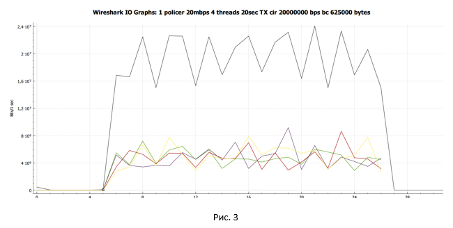
The black line shows the total traffic. The multicolored lines are the traffic of each TCP stream. Before drawing any conclusions and going into the question, let's see what we can do if we replace the policer with a shaper.
Set up a shaper at a speed limit of 20 Mbps.
Device configuration
When setting up, we use the automatic billing size of the bucket size of tokens BC and BE equal to 8000. But we change the queue size from 83 (default in IOS XE 15.6 (1) S2) to 200. This was done consciously in order to get a clearer picture typical of shaper 'but. We will dwell on this question in more detail in the subcategory “Does the queue depth affect our session?”.
policy-map Shaper_20 class class-default shape average 20000000 queue-limit 200 packets interface GigabitEthernet0/0/1 service-policy output Shaper_20 When setting up, we use the automatic billing size of the bucket size of tokens BC and BE equal to 8000. But we change the queue size from 83 (default in IOS XE 15.6 (1) S2) to 200. This was done consciously in order to get a clearer picture typical of shaper 'but. We will dwell on this question in more detail in the subcategory “Does the queue depth affect our session?”.
cbs-rtr-4000#sh policy-map interface gigabitEthernet 0/0/1 Service-policy output: Shaper_20 Class-map: class-default (match-all) 34525 packets, 50387212 bytes 5 minute offered rate 1103000 bps, drop rate 0000 bps Match: any Queueing queue limit 200 packets (queue depth/total drops/no-buffer drops) 0/0/0 (pkts output/bytes output) 34525/50387212 shape (average) cir 20000000, bc 80000, be 80000 target shape rate 20000000 In iPerf, we start generating traffic within four threads using the TCP protocol.
C:\Users\user>iperf3.exe -c 192.168.115.2 -t 20 -i 20 -P 4 Connecting to host 192.168.115.2, port 5201 [ 4] local 192.168.20.8 port 62104 connected to 192.168.115.2 port 5201 [ 6] local 192.168.20.8 port 62105 connected to 192.168.115.2 port 5201 [ 8] local 192.168.20.8 port 62106 connected to 192.168.115.2 port 5201 [ 10] local 192.168.20.8 port 62107 connected to 192.168.115.2 port 5201 [ ID] Interval Transfer Bandwidth [ 4] 0.00-20.00 sec 11.6 MBytes 4.85 Mbits/sec [ 6] 0.00-20.00 sec 11.5 MBytes 4.83 Mbits/sec [ 8] 0.00-20.00 sec 11.5 MBytes 4.83 Mbits/sec [ 10] 0.00-20.00 sec 11.5 MBytes 4.83 Mbits/sec [SUM] 0.00-20.00 sec 46.1 MBytes 19.3 Mbits/sec The average speed was 19.3 Mbit / s. In addition, each TCP stream received approximately the same bandwidth.
With Wireshark, we collect a traffic dump and build a data transfer schedule received on the sender side.
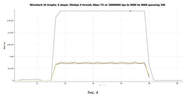
The black line shows the total traffic. The multicolored lines are the traffic of each TCP stream.
We make the first intermediate conclusions:
- In the case of policer, the usable bandwidth was 17.1 Mbps. Each stream at different points in time had a different bandwidth.
- In the case of shaper, the usable bandwidth was 19.3 Mbit / s. All streams had approximately the same bandwidth.
Let us look in more detail at the behavior of the TCP session in the case of policer and shaper. Fortunately, there are enough tools in Wireshark to make such an analysis.
Let's start with graphs that show packets with reference to the time of their transfer. The first one is policer, the second one is shaper.
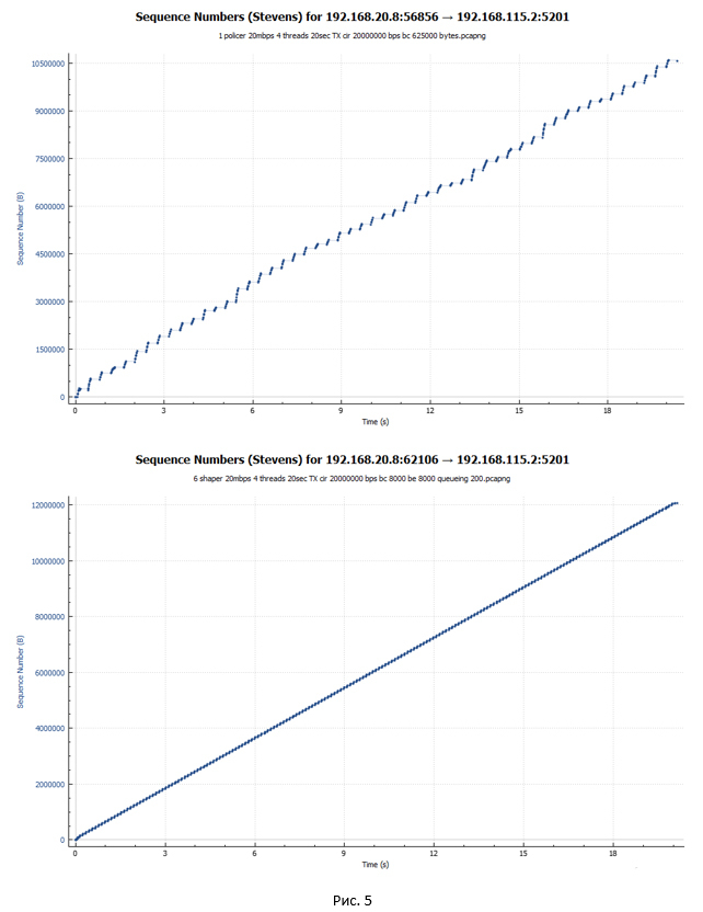
From the graphs it can be seen that the packets in the case of shaper are transmitted more evenly in time. In the case of a policer, abrupt accelerations of the session and periods of pauses are visible.
TCP session analysis with policer operation
Let's take a closer look at the TCP session. We will consider the case of policer.
TCP in its work relies on a fairly large set of algorithms. Among them, the most interesting for us are the algorithms responsible for congestion control. They are responsible for the speed of data transmission within the session. The PC running iPerf runs on Windows 10. In Windows 10, Compound TCP (CTCP) is used as such an algorithm. CTCP in its work borrowed quite a lot from the TCP Reno algorithm. Therefore, when analyzing a TCP session, it is quite convenient to look at the picture with the session states when the TCP Reno algorithm is running.
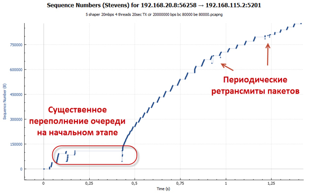
The following picture shows the initial data transfer segment.
- At the first stage, we establish a TCP session (a triple handshake takes place).
- Next starts TCP session overclocking. TCP slow-start algorithm works. By default, the congestion window (cwnd) value for a TCP session in Windows 10 is equal to the volume of ten maximum TCP session data segments (MSS). This means that this PC can send 10 packets at once, without waiting for confirmation of them in the form of an ACK. The value of the maximum window, which the recipient provided (advertised window - awnd), is taken as the initial value of the slow-start (ssthresh) algorithm termination threshold and the transition to congestion avoiding mode. In our case, ssthresh = awnd = 64K. Awnd is the maximum value of the data that the receiver is ready to receive into the buffer.Where to see the initial session data?To see the TCP options, you can use PowerShell.
We look at which global TCP template is used by default in our system.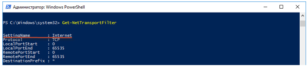
Next, execute the “Get-NetTCPSetting Internet” query and look for the value of the InitialCongestionWindow (MSS) value.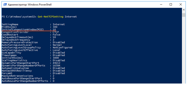
The awnd value can be found in the ACK packets received from the receiver: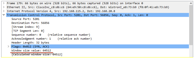
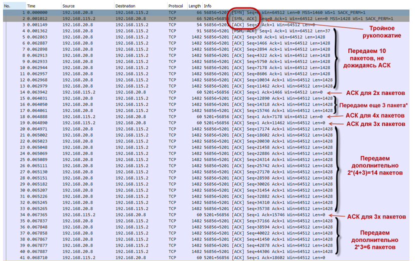
In TCP mode, the slow-start window size (cwnd) increases each time an ACK is received. However, it cannot exceed the value of awnd. Due to this behavior, we have an almost exponential increase in the number of transmitted packets. Our TCP session accelerates quite aggressively.TCP packet transmission slow-start- The PC establishes a TCP connection (# 1-3).
- Sends 10 packets (# 4-13), without waiting for confirmation (ACK), since cwnd = 10 * MSS.
- Receives ACK (№14), which confirms immediately two packages (№4-5).
- Increases window size Cwnd = (10 + 2) * MSS = 12 * MSS.
- Sends an additional three packets (# 15-17). In theory, the PC should have sent four packets: two, since it received confirmation for two packets that had been transmitted earlier; plus two packages due to the increase in the window. But in reality, at the very first stage, the system sends (2N-1) packets. I could not find the answer to this question. If someone tells me, I will be grateful.
- Receives two ACKs (# 18-19). The first ACK confirms that the remote side has received four packets (No. 6-9). The second - three (№ 10-12).
- Increases window size Cwnd = (12 + 7) * MSS = 19 * MSS.
- Sends 14 packets (# 20-33): seven new packets, since they received ACK to seven previously transmitted packets, and another seven new packets, as the window increased.
- And so on.
- Policer does not prevent the session from being overclocked. There are many tokens in the bucket (when policer is initialized, the bucket is filled with tokens completely). For a speed of 20 Mbps, the bucket size is set to 625,000 bytes by default. Thus, the session accelerates at a point in time to almost 18 Mbit / s (and we remember that we have four such sessions). The window size cwnd reaches its maximum value and becomes equal to awnd, which means cwnd = ssthersh.cwnd = ssthershWhen cwnd = ssthersh had an exact answer, I could not find whether the algorithm would change from slow-start to congestion avoidance. RFC does not give an exact answer. From a practical point of view, this is not very important, since the window size cannot continue to grow.
- Since our session accelerated quite strongly, the tokens are very quickly spent and ultimately end. The bucket does not have time to fill (filling with tokens goes for a speed of 20 Mbit / s, while the total utilization of all four sessions at a time point approaches 80 Mbit / s). Policer starts to drop packets. So, they do not reach the remote side. The recipient sends Duplicate ACK (Dup ACK), which signal to the sender that there has been a loss of packets and need to transfer them again.
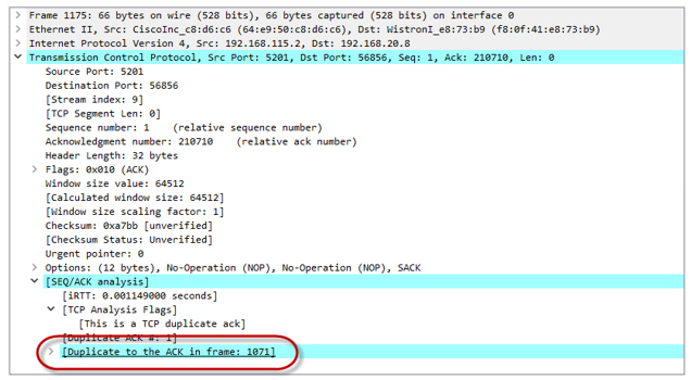
After receiving three Dup ACKs, our TCP session enters the recovery after loss phase (loss recovery, including Fast Retransmit / Fast Recovery algorithms). The sender sets the new value ssthresh = cwnd / 2 (32K) and makes the window cwnd = ssthresh + 3 * MSS.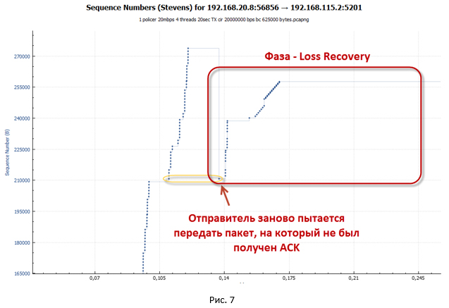
- The sender tries to immediately begin to re-transmit the lost packets (TCP Fast Retransmission algorithm works). At the same time, Dup ACKs continue to arrive, the purpose of which is to artificially increase the cwnd window. This is necessary to restore the session speed due to packet loss as quickly as possible. Due to the Dup ACK, the cwnd window grows to the maximum value (awnd).
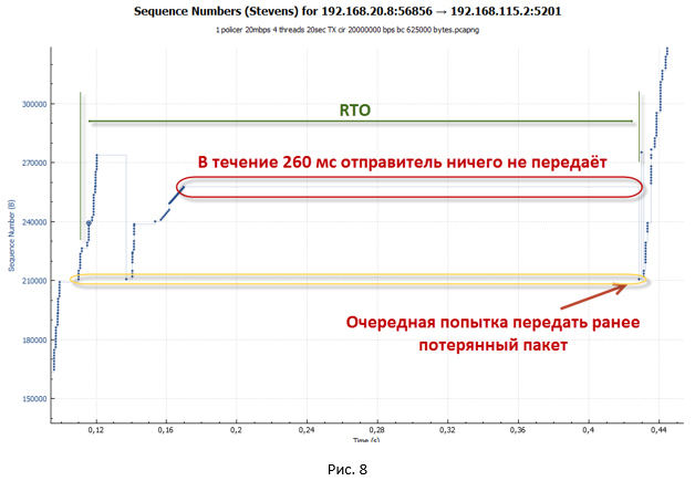
As soon as the number of packets sent to the cwnd window has been sent, the system stops. To continue data transfer, it needs new ACK (not Dup ACK). But ACK do not come. All repeated packets are discarded by policer, so the tokens in the bucket are over, and too little time has passed to fill them up. - In this state, the system waits until the timeout for receiving a new ACK from the remote side (Retransmission timeout - RTO ) works. Our big pauses, which are visible on the charts, are connected with this.
- After the RTO timer is triggered, the system goes into slow-start mode and sets ssthresh = FlightSize / 2 (where FlightSize is the amount of not confirmed data), and the window cwnd = 1 * MSS. Then again, an attempt is made to transfer the lost packets. However, now only one packet is being sent, since cwnd = 1 * MSS.
- Since for some time the system did not transmit anything, tokens managed to accumulate in our bucket. Therefore, in the end, the package reaches the recipient. So, we get a new ACK. From this moment on, the system starts transmitting previously lost packets in slow-start mode. The session is being overclocked. As soon as the window size cwnd exceeds the value of ssthresh, the session goes into congestion avoidance mode.
In the Compound TCP algorithm, the sending window (wnd) is used to control the transmission rate, which depends on two weighted values: the overload window (cwnd) and the delay window (dwnd). Cwnd, as before, depends on the received ACK, dwnd depends on the amount of round trip time (RTT). The wnd window only grows once per RTT time period. As we remember, in the case of slow-start, the cwnd window grew when each ACK was received. Therefore, in congestion avoidance mode, the session is not accelerated so quickly. - As soon as the session accelerates strongly enough (when more packets are transferred than there are tokens in the bucket), the policer is triggered again. Begin to drop packets. Next comes the loss recovery phase. Those. the whole process is repeated again. And so it goes until we have completed the transfer of all data.
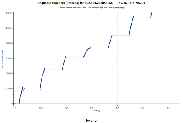
TCP session during policer operation looks like a ladder (the transmission phase goes, followed by a pause).
TCP session analysis when running shaper
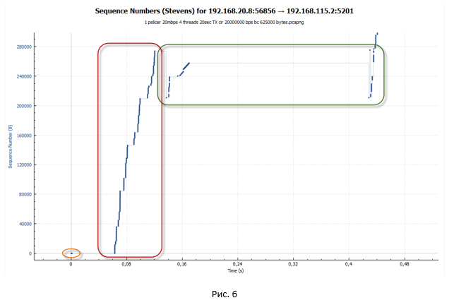
Now let's take a closer look at the data segment for the shaper case. For clarity, let's take a similar scale, as for the policer graph in Fig.6.
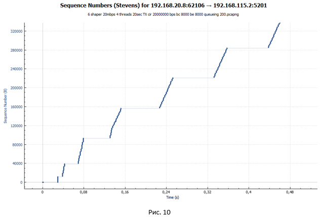
From the graph we see the same ladder. But the size of the steps was significantly smaller. However, if you look closely at the graph in Fig. 10, we will not see small “waves” at the end of each step, as was the case in Fig. 9. Such “waves” were the result of packet loss and retransmission attempts.
Consider the initial data transfer segment for the shaper case.
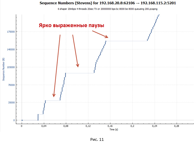
The session is established. Next begins slow-start TCP overclocking. But this acceleration is flatter and has pronounced pauses that increase in size. Flatter overclocking is due to the fact that the default bucket size for shaper is all (BC + BE) = 20,000 bytes. While for a policer, the bucket size is 625,000 bytes. Therefore, the shaper works significantly earlier. Packages begin to fall into the queue. The delay from the sender to the receiver grows, and ACKs arrive later than it did in the case of the policer. The window grows much slower. It turns out that the more the system transmits packets, the more they accumulate in the queue, and therefore, the greater the delay in receiving the ACK. We have a process of self-regulation.
After a while, the cwnd window reaches the awnd value. But at this point, we have accumulated quite a noticeable delay due to the presence of the queue. Ultimately, when a certain RTT value is reached, an equilibrium state occurs, when the session rate does not change any more and reaches a maximum value for this RTT. In my example, the average RTT is 107 ms, awnd = 64512 bytes, therefore, the maximum session speed will correspond to awnd / RTT = 4.82 Mbit / s. Approximately this value gave us iPerf during measurements.
But where are the pronounced pauses in the transmission? Let's look at the schedule of packet transmission through the device with a shaper in case we have only one TCP session (Figure 12). Let me remind you that in our experiment, data transfer occurs within four TCP sessions.
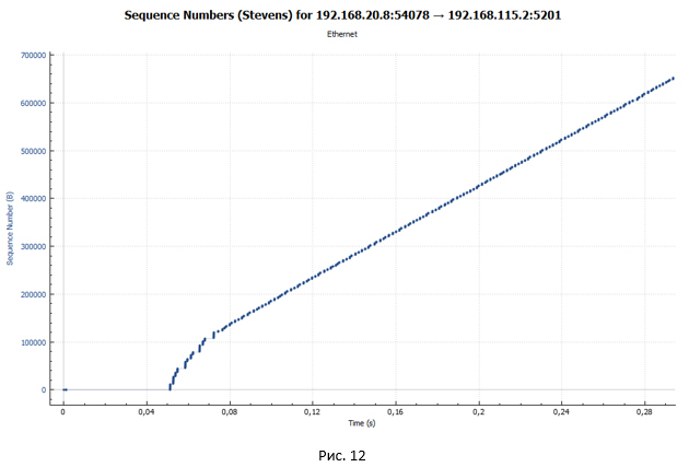
This graph shows very clearly that there are no pauses. From this we can conclude that the pauses in Fig.10 and 11 are due to the fact that we simultaneously have four streams, and the queue in the shaper is one (the type of the FIFO queue).
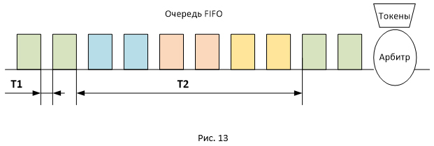
Figure 13 shows the location of the packets of different sessions in the FIFO queue. Since packets are transmitted in batches, they will be queued in the same way. In this regard, the delay between the arrival of packets on the receiving side will be of two types: T1 and T2 (where T2 is significantly superior to T1). The total RTT value for all packets will be the same, but packets will arrive in batches spaced apart in time by the value of T2. So pauses are obtained, since at the time T2 no ACKs come to the sender, while the session window remains unchanged (has a maximum value equal to awnd).
WFQ Queue
It is logical to assume that if we replace one common FIFO queue with several for each session, there will not be any pronounced pauses. For such a problem, for example, a queue of type Weighted Fair Queuing ( WFQ ) is suitable . It creates its own queue of packets for each session.
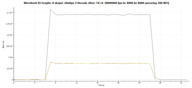
From the general graph, we immediately see that the graphs of all four TCP sessions are identical. Those. they all got the same bandwidth.
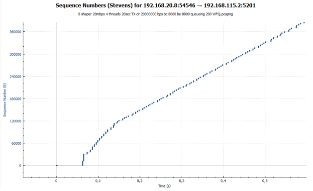
And here is our schedule of packet distribution over transmission time at exactly the same scale as in Fig. 11. There are no pauses.
It is worth noting that the WFQ queue will allow us to get not only a more even distribution of bandwidth, but also to prevent the "clogging" of one type of traffic by another. We talked all the time about TCP, but UDP traffic is also present on the network. UDP has no mechanisms for adjusting the rate of transmission (flow control, congestion control). Because of this, UDP traffic can easily clog our shared FIFO queue in a shaper, which will dramatically affect TCP transmission. Let me remind you that when the FIFO queue is completely full of packets, the tail-drop mechanism starts working by default, in which all newly arrived packets are discarded. If we have a WFQ queue configured, each session waits for buffering in its turn, which means that TCP sessions will be separated from UDP sessions.
policy-map Shaper class shaper_class shape average 20000000 queue-limit 200 packets fair-queue From the general graph, we immediately see that the graphs of all four TCP sessions are identical. Those. they all got the same bandwidth.
And here is our schedule of packet distribution over transmission time at exactly the same scale as in Fig. 11. There are no pauses.
It is worth noting that the WFQ queue will allow us to get not only a more even distribution of bandwidth, but also to prevent the "clogging" of one type of traffic by another. We talked all the time about TCP, but UDP traffic is also present on the network. UDP has no mechanisms for adjusting the rate of transmission (flow control, congestion control). Because of this, UDP traffic can easily clog our shared FIFO queue in a shaper, which will dramatically affect TCP transmission. Let me remind you that when the FIFO queue is completely full of packets, the tail-drop mechanism starts working by default, in which all newly arrived packets are discarded. If we have a WFQ queue configured, each session waits for buffering in its turn, which means that TCP sessions will be separated from UDP sessions.
The most important conclusion that can be made after analyzing the packet transfer schedules when working with a shaper is that we do not have any lost packets. Due to the increase in RTT, the session speed adapts to the speed of the shaper.
Does the queue depth affect our session?
Of course! Initially (if someone still remembers this) we changed the queue depth from 83 (the default value) to 200 packets. We did this in order to have enough queues to get a sufficient RTT value, at which the total speed of the sessions becomes approximately equal to 20 Mbps. So, the packages "do not fall out" from the shaper'a queue.
At a depth of 83 packets, the queue overflows faster than the desired RTT value is reached. Packets are discarded. This is especially vivid at the initial stage, when the TCP slow-start mechanism works for us (the session accelerates as aggressively as possible). It is worth noting that the number of discarded packets is incomparably smaller than in the case of policer, since an increase in RTT causes the session speed to grow more smoothly. As we remember, in the CTCP algorithm, the window size also depends on the RTT value.
At a depth of 83 packets, the queue overflows faster than the desired RTT value is reached. Packets are discarded. This is especially vivid at the initial stage, when the TCP slow-start mechanism works for us (the session accelerates as aggressively as possible). It is worth noting that the number of discarded packets is incomparably smaller than in the case of policer, since an increase in RTT causes the session speed to grow more smoothly. As we remember, in the CTCP algorithm, the window size also depends on the RTT value.
Bandwidth utilization and latency charts for policer and shaper
In conclusion of our small research we will construct several more general graphs, after which we proceed to the analysis of the data obtained.
Bandwidth utilization schedule:
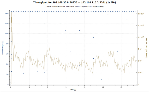
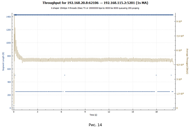
In the case of a policer, we see a hopping schedule: the session accelerates, then losses occur, and its speed drops. Then everything repeats again. In the case of shaper, our session receives approximately the same bandwidth throughout the transmission. Session speed is adjusted by increasing the RTT value. In both graphs, explosive growth can be observed initially. It is due to the fact that our buckets were initially completely filled with tokens and the TCP session, unrestrained, is accelerated to relatively large values (in the case of shaper, this value is 2 times less).
Schedule RTT delay for policer and shaper (in a good way, this is the first thing we remember when talking about shaper):
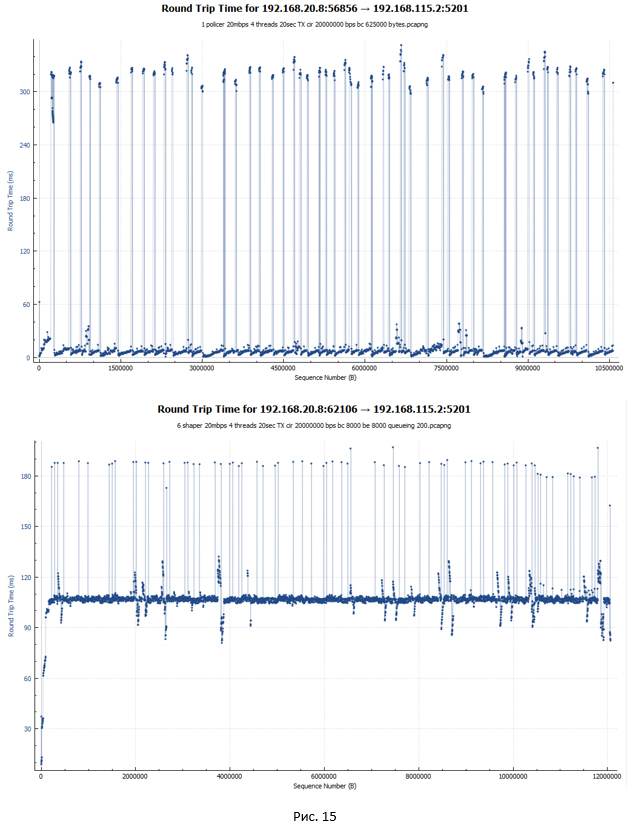
In the case of a policer (first graph), the RTT delay for most packets is minimal, about 5 ms. The graph also contains significant jumps (up to 340 ms). These are the moments when the packets were discarded and transmitted again. Here it is worth noting how Wireshark considers RTT for TCP traffic. RTT is the time between sending an original packet and receiving an ACK on it. In this regard, if the original packet was lost and the system re-transmitted the packet, the RTT value grows, since the starting point is in any case the moment of sending the original packet.
In the case of shaper, the RTT delay for most packets was 107 ms, since they all linger in the queue. There are peaks up to 190 ms.
findings
So, what final conclusions can be made. Someone may notice that this is so clear. But our goal was to dig a little deeper. Let me remind you that the experiment analyzed the behavior of TCP sessions.
- Shaper 13% , policer (19.3 17.1 /) 20 /.
- shaper' . WFQ. policer' .
- shaper' (, ). policer' – 12.7%.
policer , , policer'. , , . - shaper' ( – 102 ). , , shaper' (jitter) . , jitter.
– ( Bufferbloat ). . - shaper . , . policer' , .
- Policer shaper , UDP «» TCP. .
- shaper' , policer'. .
One more fact can be noted, though not directly related to the speed limitation task. Shaper allows us to configure various types of queues (FIFO, WFQ, etc.), thus providing various levels of traffic prioritization when sending it through the device. This is very convenient in cases where the actual speed of traffic transmission differs from the channel one (for example, this often happens with Internet access or WAN channels).
The study of the impact of policer on the Internet
Google , policer' . , 2% 7% policer'. policer' 21%, 6 , , . , policer', , , policer .
policer' .
-:
shaper . Shaper , ( BC = 8 000 ). . , . .
- , policer'. . — TCP: TCP Pacing ( RTT, ACK) loss recovery ( ACK ).
policer' .
-:
- policer' (burst size). , TCP , , .
- policer' shaper ( ).
- shaper, policer . shaper , policer. Shaper , . - policer , . .
shaper . Shaper , ( BC = 8 000 ). . , . .
- , policer'. . — TCP: TCP Pacing ( RTT, ACK) loss recovery ( ACK ).
Thus, there is no definitive answer to the question which is better to use: shaper or policer. Each technology has its pros and cons. For some, the additional delay and the load on the equipment is not as critical as for the other. So the choice is made in the direction of shaper. For some, it is important to minimize network buffering to fight jitter - this means our policer technology. In some cases, both technologies can be used simultaneously. Therefore, the choice of technology depends on each specific situation in the network.
Source: https://habr.com/ru/post/317048/
All Articles