We write real Pointer Analysis for LLVM. Part 1: Introducing or first meeting with the world of program analysis
 Hi, Habr!
This article will be introductory in my short series of notes on a program analysis technique such as pointer analysis. Algorithms of pointer analysis allow with a given accuracy to determine which parts of the memory a variable or an expression can indicate. Without knowledge of information about pointers, the analysis of programs that actively use pointers (that is, programs in any modern programming language — C, C ++, C #, Java, Python, and others) —is virtually impossible. Therefore, in any more or less optimizing compiler or serious static code analyzer, pointer analysis techniques are used to achieve accurate results.
In this series of articles, we will focus on writing an effective interprocedural pointer analysis algorithm, consider the main modern approaches to the problem, and, of course, we will write our very serious pointer analysis algorithm for the wonderful language of the internal presentation of LLVM programs. I ask all those who are interested under the cat, we will analyze the program and much more!
Algorithms for optimization and analysis of programs
Imagine for a moment that you are writing a compiler for your favorite programming language. Behind the writing of lexical and syntactic analyzers, the syntax tree of the translation module has already been built and the source program is written in terms of some internal representation (for example, in the form of JVM bytecode or LLVM). What's next? You can, for example, try to interpret the received representation on some virtual machine, or translate this representation further, already into machine code. And you can first try to optimize this presentation, and then do a boring broadcast, right? In addition, the program will work faster!
')
What optimizations can we apply? Consider, for example, such a code snippet.
k = 2; if (complexComputationsOMG()) { a = k + 2; } else { a = k * 2; } if (1 < a) { callUrEx(); } k = complexComputationsAgain(); print(a); exit(); Note that the variable
a takes a value of 4 , regardless of what value the complexComputationsOMG function complexComputationsOMG , which means that the call to this function can be safely removed from the program view (assuming that all the functions are clean in particular, do not have side effects). Moreover, since at the point of the program where the variable a is compared with the unit, the variable a always takes the value 4 , the callUrEx can be called unconditionally, that is, it can get rid of unnecessary branching.In addition, the value of the variable
k , assigned in the line k = complexComputationsAgain() not used anywhere, so this function can not be called! This is what we get after all the transformations. callUrEx(); print(4); exit(); In my opinion, not bad! All we have to do is to teach our optimizer to perform such code transformations automatically. Here we are helped by all the variety of dataflow analysis algorithms, and very cool guy Gary Kildall , who in his monumental manuscript “A unified approach to global program optimization” presented a universal framework for analyzing programs, more precisely the so-called dataflow problems.
Descriptively, an iterative solution to the dataflow problems, sounds very simple. All we need is to define a set of properties of variables that we want to monitor during the analysis (for example, possible values of variables), functions for interpreting such sets for each base block, and the rules by which we will distribute these properties between base blocks (for example, the intersection sets). During the iterative algorithm, we calculate the values of these variable properties at different points in the control flow graph ( CFG ), usually at the beginning and end of each base unit. Iteratively spreading these properties, we must eventually reach a fixed point (fixpoint), in which the algorithm finishes its work.

Of course, it’s better to see once than to hear a hundred times, so let's back up the words with an example. Consider the following code snippet and try to track the possible values of variables at various points in the program.
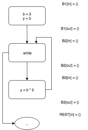
b = 3; y = 5; while (...) { y = b * 2; } if (b < 4) { println("Here we go!"); } The box below solves the classical problem of program analysis, namely, the propagation of constants (constant propagation) for the considered code fragment.
Iterative algorithm of constant propagation
At the beginning, all sets of possible values of variables are empty.
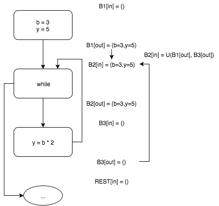
Interpreting the input block

The loop entry block in
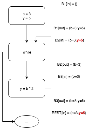
At the output of the base unit

Since the information about the possible values of the variables has been changed (compared to the initial state, that is, as if by the 0th iteration of the algorithm), we start the next iteration of the algorithm. The new iteration repeats the previous one except for the step of calculating the input set of block
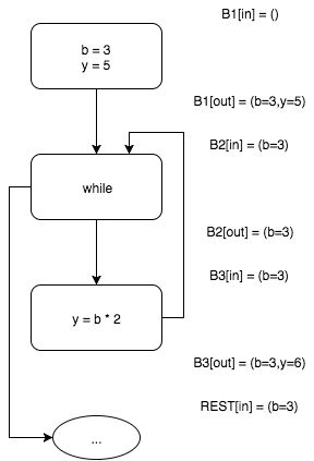
As we see, this time we are forced to “cross” the output sets of blocks
Since continuing the calculations further we do not get any new values, the work of the algorithm can be considered complete. This means that we have reached a fixed point.
Interpreting the input block
B1 , we find that the output of this block is b=3 and y=5 . The function f1 (similar functions are defined for the remaining blocks) is the function of the interpretation of the block.The loop entry block in
while B2 has two ancestors - the input block B1 and the block B3 . Since the B3 block does not yet contain the possible values of the variables, at the current stage of the algorithm we assume that b=3 and y=5 at the input and output of the block. The function U is the rule of propagation of sets of properties of variables (usually the exact lower bound of a partially ordered set, or more precisely, a complete lattice ).At the output of the base unit
B3 - b=3 and y=6 .Since the information about the possible values of the variables has been changed (compared to the initial state, that is, as if by the 0th iteration of the algorithm), we start the next iteration of the algorithm. The new iteration repeats the previous one except for the step of calculating the input set of block
B2 .As we see, this time we are forced to “cross” the output sets of blocks
B1 and B3 . These sets have a common part b=3 that we leave and the different parts y=5 and y=6 , which we have to drop.Since continuing the calculations further we do not get any new values, the work of the algorithm can be considered complete. This means that we have reached a fixed point.
In his work, Gary Kildall showed that such an iterative algorithm will always complete its work and, moreover, give the fullest possible results if the following conditions are met:
- the domain of tracked variable properties is a complete lattice;
- the block interpretation function has the property of distributivity on the lattice;
- for the “meeting” of the base blocks of the precedents, the exact lower bound operator is used (that is, the meet function of the partially ordered set).
Anecdote from the world of big science
The funny thing is that the example that Kildall used in his work (constant propagation) does not satisfy the requirements that he also makes to the dataflow problem - the interpretation functions for constant propagation do not have the distributivity property on the lattice, but are only monotonic.
Thus, to optimize programs, we can use the full power of dataflow analysis algorithms, using, for example, an iterative algorithm. Returning to our first example, we used constant propagation and liveness analysis (live variable analysis) to perform dead code elimination optimization.
Moreover, dataflow analysis algorithms can be used when performing static code analysis in the context of information security. For example, in the process of searching for vulnerabilities of the SQL-injection class, we can mark with a special flag all variables that could be affected in any way by an attacker (for example, HTTP request parameters, etc.). If it turns out that a variable marked with such a flag participates in the formation of a SQL query without proper processing - we most likely found a serious security hole in the application! It will only show a message about possible vulnerabilities and
Multiply grief
Ivan nods at Peter, and Peter at Ivan
Summing up the previous paragraph, dataflow analysis algorithms are the daily bread (and butter!) Of any compiler. So where is the pointer analysis, and why is it really needed?
I hasten to spoil your mood with the following example.
x = 1; *p = 3; if (x < 3) { killTheCat(); } Obviously, not knowing where the variable
p points to, we cannot say with certainty what the value of the expression x < 3 in the conditional if will equal. The answer to this question we can give only by finding out the context in which the given code fragment appears. For example, p can be a global variable from another module (which in the C programming languages can point to anything and anytime) or a local variable pointing somewhere in the heap. Even knowing the context, we still need to know the many locations (abstract memory cells) that this variable can point to. If, for example, before the specified code fragment, the variable p initialized as p = new int , then we must remove the conditional killTheCat from the optimized program and call the killTheCat method unconditionally.If so, we will not be able to apply any optimization to this code until we find any way to find out once and for all where the variables in the analyzed program can point!
I think it has already become obvious that we cannot do without the use of pointer analysis (and for what reason did it become necessary to solve this complex, or rather, algorithmically unsolvable task). Pointer analysis is a static code analysis method that determines information about the values of pointers or expressions of the pointer type. Depending on the tasks being solved, pointer analysis can determine information for each point of the program or for the program as a whole (flow-sensitivity) or depending on the context of the function call (context-sensitivity). I will tell you more about pointer analysis types in one of the following articles in the series.
The result of the analysis is usually represented as a mapping from a set of pointers to a set of locations to which these pointers can refer. That is, simply put, each pointer
p assigned a set of objects to which it can point. For example, in the code snippet below, the result of the analysis will be the mapping p -> {a, b}, q -> {p} . int a, b, c, *p, **q; p = &a; q = &p; *q = &b; It is important to note that the mapping calculated by pointer analysis must meet the security criterion, that is, be as conservative as possible. Otherwise, we can simply spoil the semantics of the source program by our optimizations. For example, a safe approximation of the pointer analysis result for the program fragment above may be
p -> {a, b, c}, q -> {unknown} . The value unknown used to indicate that the pointer can refer to all available program objects.For example, in the code snippet considered below, dereferencing the variable
p can potentially change the value of any program object! extern int *offensiveFoo(); p = offensiveFoo(); *p = 77; We do not know anything about the
offensiveFoo function, since it was imported from another broadcast module, and therefore we have to assume that p can indicate absolutely anything!In the following, we will assume that all the functions and global variables under consideration belong to the broadcast module being analyzed, unless the reverse is explicitly discussed with words.
Poor Man's Pointer Analysis
 Having faced the problem of aliasing pointers for the first time, I, without hesitation, decided to try to solve the problem using the already known iterative algorithm on the grid (then I had no idea that I was solving the same problem as the pointer analysis algorithms solve). Indeed, what prevents us from tracking objects that pointers can refer to as a set of properties of these pointers? Let's try to track the work of the algorithm on a simple example. Let the rules for the propagation of sets of objects correspond to the “natural” semantics of the program (for example, if
 p = &a , then p -> {a} ), and distribute these sets between the basic blocks we will be simply joining sets (for example, if q -> {a, b} and q -> {c} are input to some base unit, then the input set for such a block will be q -> {a, b, c} ).Consider the work of the algorithm on a simple example.
x = &a; a = &z; if (...) { x = &b; } else { c = &x; } Wait until the iterative algorithm finishes and look at the results.
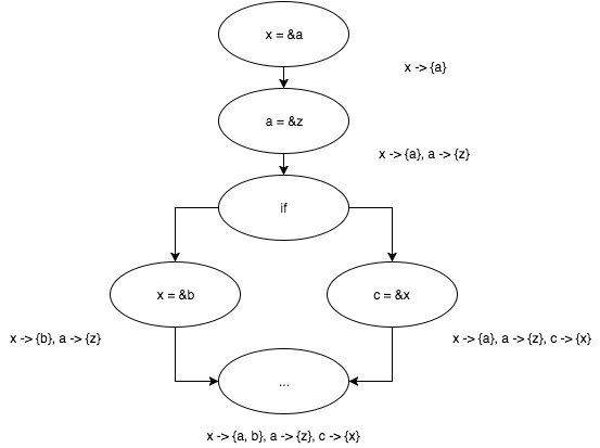
Works! Despite the simplicity of the algorithm, the presented approach has the right to life. I would say more precisely that it was (of course, with significant improvements) that the aliasing of pointers was solved before the appearance of Andersen’s Program Analysis and Specialization for the C Programming Language. By the way, the next article of the cycle will be devoted to this work!
The main disadvantages of the described approach are poor scalability and too conservative results, since the analysis of real programs must take into account the challenges of other functions (that is, the analysis must be interprocedural) and, often, the context of the function call. The essential advantage of this approach is that the information about the pointers is available for each point of the program (that is, the flow-sensitive algorithm), while the algorithms of Andersen and his followers calculate the result for the program as a whole (flow-insensitive).
Instead of conclusion

This concludes the first piece of my cycle of notes about pointer analysis algorithms. Next time we will write a simple and efficient interprocedural pointer analysis algorithm for LLVM!
Thank you all very much for your time!
Source: https://habr.com/ru/post/317002/
All Articles