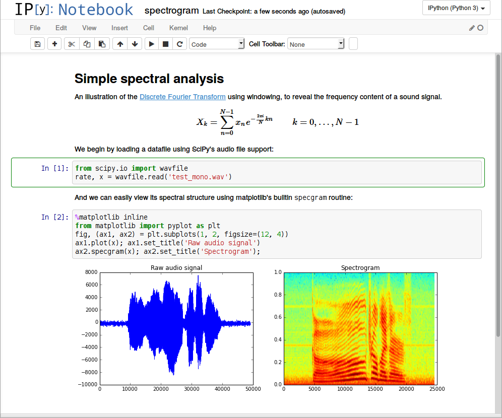
Jupyter Notebook features that you may not have heard of

Jupyter Notebook is an extremely handy tool for creating beautiful analytical reports, as it allows you to store together code, images, comments, formulas and graphs:



Below we will talk about some of the features that make Jupyter very cool. You can read about them in other places, but if you don’t specifically ask this question, you will never read it.

Jupyter supports many programming languages ​​and can be easily run on any server, only access via ssh or http is necessary. In addition, it is free software.
')

The basics

You can find a list of hotkeys in Help> Keyboard Shortcuts (the list is periodically updated, so feel free to look in there again).

From here you can get an idea of ​​the interaction with the notebook (notebook). If you will be constantly working with Jupyter, most of the combinations you will quickly learn.

For example,

• Esc + F will find and replace only in the code, not taking into account the output;
• Esc + O - switch to the cell output;
• You can select several cells at once and delete / copy / cut / paste. This is useful if you need to move parts of a notebook.

Export Notepad

The simplest way is to save the notebook in IPython Notebook format (.ipynb), but since not all of them are used, there are other options:

• Convert notepad to html-file;
• Post it to gists , which can handle files of this format ( see example );
• Save your notebook, for example, in the dropbox, and then open the link in nbviewer ;
• Notepads can open github (there are some limitations, but in most cases it works), which is very useful because it allows you to store the history of the study (if the study is available to the general public).

Plotting

There are several options for plotting graphs:

• matplotlib (actually, stardart), enabled by the command %matplotlib inline ;
• %matplotlib notebook is an interactive mode, but it works very slowly, since the graphics are processed on the server side;
• mpld3 is an alternative visualization library (using D3) for matplotlib. She is pretty good, although incomplete.
• bokeh is better suited for building interactive graphs;
• plot.ly builds beautiful graphics, but it will cost money.

Magic commands

Magic commands (magics) turn an ordinary python into a magical python . Magic commands are the key to IPython's power.

 # list available python magics %lsmagic 

 Available line magics: %alias %alias_magic %autocall %automagic %autosave %bookmark %cat %cd %clear %colors %config %connect_info %cp %debug %dhist %dirs %doctest_mode %ed %edit %env %gui %hist %history %killbgscripts %ldir %less %lf %lk %ll %load %load_ext %loadpy %logoff %logon %logstart %logstate %logstop %ls %lsmagic %lx %macro %magic %man %matplotlib %mkdir %more %mv %notebook %page %pastebin %pdb %pdef %pdoc %pfile %pinfo %pinfo2 %popd %pprint %precision %profile %prun %psearch %psource %pushd %pwd %pycat %pylab %qtconsole %quickref %recall %rehashx %reload_ext %rep %rerun %reset %reset_selective %rm %rmdir %run %save %sc %set_env %store %sx %system %tb %time %timeit %unalias %unload_ext %who %who_ls %whos %xdel %xmode Available cell magics: %%! %%HTML %%SVG %%bash %%capture %%debug %%file %%html %%javascript %%js %%latex %%perl %%prun %%pypy %%python %%python2 %%python3 %%ruby %%script %%sh %%svg %%sx %%system %%time %%timeit %%writefile Automagic is ON, % prefix IS NOT needed for line magics. 

% env

You can manage the environment variables for your notepad without restarting the Jupyter server. Some libraries (such as theano) use environment variables to control behavior, and% env is the most convenient way.

 #%env - without arguments lists environmental variables %env OMP_NUM_THREADS=4 

 env: OMP_NUM_THREADS=4 

Execution of shell commands

In Notebook, you can call any shell command. This is especially useful for managing a virtual environment.

 !pip install numpy !pip list | grep Theano 

 Requirement already satisfied (use --upgrade to upgrade): numpy in /Users/axelr/.venvs/rep/lib/python2.7/site-packages Theano (0.8.2) 

Suppress last line output

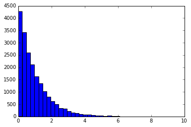
Sometimes the output is not needed, and in this case, you can either use the pass command from a new line, or put a comma at the end of the line:

 %matplotlib inline from matplotlib import pyplot as plt import numpy 

 # if you don't put semicolon at the end, you'll have output of function printed plt.hist(numpy.linspace(0, 1, 1000)**1.5); 

View the source of functions / classes / anything with a question mark (?, ??)

 from sklearn.cross_validation import train_test_split # show the sources of train_test_split function in the pop-up window train_test_split?? 

 # you can use ? to get details about magics, for instance: %pycat? 

will bring up the following popup window:

 Show a syntax-highlighted file through a pager. This magic is similar to the cat utility, but it will assume the file to be Python source and will show it with syntax highlighting. This magic command can either take a local filename, an url, an history range (see %history) or a macro as argument :: %pycat myscript.py %pycat 7-27 %pycat myMacro %pycat http://www.example.com/myscript.py 

Use% run to execute Python code.

% run can execute Python code from files with the .py extension — this behavior is well documented.

But this command can execute other notebooks from Jupyter! Sometimes it is very useful.

Note that% run is not the same as importing a python module.

 # this will execute all the code cells from different notebooks %run ./2015-09-29-NumpyTipsAndTricks1.ipynb 

 [49 34 49 41 59 45 30 33 34 57] [172 177 209 197 171 176 209 208 166 151] [30 33 34 34 41 45 49 49 57 59] [209 208 177 166 197 176 172 209 151 171] [1 0 4 8 6 5 2 9 7 3] ['a' 'b' 'c' 'd' 'e' 'f' 'g' 'h' 'i' 'j'] ['b' 'a' 'e' 'i' 'g' 'f' 'c' 'j' 'h' 'd'] ['a' 'b' 'c' 'd' 'e' 'f' 'g' 'h' 'i' 'j'] [1 0 6 9 2 5 4 8 3 7] [1 0 6 9 2 5 4 8 3 7] [ 0.93551212 0.75079687 0.87495146 0.3344709 0.99628591 0.34355057 0.90019059 0.88272132 0.67272068 0.24679158] [8 4 5 1 9 2 7 6 3 0] 

 [-5 -4 -3 -2 -1 0 1 2 3 4] [0 0 0 0 0 0 1 2 3 4] ['eh' 'cl' 'ah' ..., 'ab' 'bm' 'ab'] ['ab' 'ac' 'ad' 'ae' 'af' 'ag' 'ah' 'ai' 'aj' 'ak' 'al' 'am' 'an' 'bc' 'bd' 'be' 'bf' 'bg' 'bh' 'bi' 'bj' 'bk' 'bl' 'bm' 'bn' 'cd' 'ce' 'cf' 'cg' 'ch' 'ci' 'cj' 'ck' 'cl' 'cm' 'cn' 'de' 'df' 'dg' 'dh' 'di' 'dj' 'dk' 'dl' 'dm' 'dn' 'ef' 'eg' 'eh' 'ei' 'ej' 'ek' 'el' 'em' 'en' 'fg' 'fh' 'fi' 'fj' 'fk' 'fl' 'fm' 'fn' 'gh' 'gi' 'gj' 'gk' 'gl' 'gm' 'gn' 'hi' 'hj' 'hk' 'hl' 'hm' 'hn' 'ij' 'ik' 'il' 'im' 'in' 'jk' 'jl' 'jm' 'jn' 'kl' 'km' 'kn' 'lm' 'ln' 'mn'] [48 33 6 ..., 0 23 0] ['eh' 'cl' 'ah' ..., 'ab' 'bm' 'ab'] ['eh' 'cl' 'ah' ..., 'ab' 'bm' 'ab'] ['bf' 'cl' 'dn' ..., 'dm' 'cn' 'dj'] ['bf' 'cl' 'dn' ..., 'dm' 'cn' 'dj'] 

 [ 2.29711325 1.82679746 2.65173344 ..., 2.15286813 2.308737 2.15286813] 1000 loops, best of 3: 1.09 ms per loop The slowest run took 8.44 times longer than the fastest. This could mean that an intermediate result is being cached. 10000 loops, best of 3: 21.5 µs per loop 

 0.416 0.416 

% load

Load the code directly into the cell. You can select a file locally or from the network.

If you uncomment and execute the code below, the contents of the cell are replaced with the contents of the file.

 # %load http://matplotlib.org/mpl_examples/pylab_examples/contour_demo.py 

% store - lazy data transfer between notebooks

 data = 'this is the string I want to pass to different notebook' %store data del data # deleted variable 

 Stored 'data' (str) 

 # in second notebook I will use: %store -r data print data 

 this is the string I want to pass to different notebook 

% who to analyze global namespace variables

 # pring names of string variables %who str 

  data 

Timing

If you want to measure the execution time of a program or find a bottleneck in the code, IPython comes to the rescue.

 %%time import time time.sleep(2) # sleep for two seconds 

 CPU times: user 1.23 ms, sys: 4.82 ms, total: 6.05 ms Wall time: 2 s 

 # measure small code snippets with timeit ! import numpy %timeit numpy.random.normal(size=100) 

 The slowest run took 13.85 times longer than the fastest. This could mean that an intermediate result is being cached. 100000 loops, best of 3: 6.35 µs per loop 

 %%writefile pythoncode.py import numpy def append_if_not_exists(arr, x): if x not in arr: arr.append(x) def some_useless_slow_function(): arr = list() for i in range(10000): x = numpy.random.randint(0, 10000) append_if_not_exists(arr, x) 

 Overwriting pythoncode.py 

 # shows highlighted source of the newly-created file %pycat pythoncode.py 

 from pythoncode import some_useless_slow_function, append_if_not_exists 

Profiling:% prun,% lprun,% mprun

 # shows how much time program spent in each function %prun some_useless_slow_function() 

Example output:

 26338 function calls in 0.713 seconds Ordered by: internal time ncalls tottime percall cumtime percall filename:lineno(function) 10000 0.684 0.000 0.685 0.000 pythoncode.py:3(append_if_not_exists) 10000 0.014 0.000 0.014 0.000 {method 'randint' of 'mtrand.RandomState' objects} 1 0.011 0.011 0.713 0.713 pythoncode.py:7(some_useless_slow_function) 1 0.003 0.003 0.003 0.003 {range} 6334 0.001 0.000 0.001 0.000 {method 'append' of 'list' objects} 1 0.000 0.000 0.713 0.713 <string>:1(<module>) 1 0.000 0.000 0.000 0.000 {method 'disable' of '_lsprof.Profiler' objects} 

 %load_ext memory_profiler 

 # tracking memory consumption (show in the pop-up) %mprun -f append_if_not_exists some_useless_slow_function() 

 ('',) 

Example output:

 Line # Mem usage Increment Line Contents ================================================ 3 20.6 MiB 0.0 MiB def append_if_not_exists(arr, x): 4 20.6 MiB 0.0 MiB if x not in arr: 5 20.6 MiB 0.0 MiB arr.append(x) 

% lprun allows you to profile up to lines of code, but it seems that it does not work in the latest release of Python, so this time we'll do without magic:

 import line_profiler lp = line_profiler.LineProfiler() lp.add_function(some_useless_slow_function) lp.runctx('some_useless_slow_function()', locals=locals(), globals=globals()) lp.print_stats() 

 Timer unit: 1e-06 s Total time: 1.27826 s File: pythoncode.py Function: some_useless_slow_function at line 7 Line # Hits Time Per Hit % Time Line Contents ============================================================== 7 def some_useless_slow_function(): 8 1 5 5.0 0.0 arr = list() 9 10001 17838 1.8 1.4 for i in range(10000): 10 10000 38254 3.8 3.0 x = numpy.random.randint(0, 10000) 11 10000 1222162 122.2 95.6 append_if_not_exists(arr, x) 

Debug with% debug

Jupyter has its own interface for ipdb , which allows you to go inside the function and see what happens in it.

This is not PyCharm - it will take time to learn, but if you need debug on the server, this may be the only option (except pdb via the terminal).

 #%%debug filename:line_number_for_breakpoint # Here some code that fails. This will activate interactive context for debugging 

A slightly simpler way is with the% pdb command, which activates the debugger when an exception is thrown:

 # %pdb # def pick_and_take(): # picked = numpy.random.randint(0, 1000) # raise NotImplementedError() # pick_and_take() 

Formula Recording in LateX

Marcdown cells can draw LateX formulas using MathJax.

Markdaun is an important part of notebooks, so do not forget to use its expressive features!

Using different languages ​​within the same notebook

If you miss other programming languages, you can use them in Jupyter Notebook:

• %% python2
• %% python3
• %% ruby
• %% perl
• %% bash
• %% R,

but, of course, the environment must be configured accordingly.

 %%ruby puts 'Hi, this is ruby.' 

 Hi, this is ruby. 

 %%bash echo 'Hi, this is bash.' 

 Hi, this is bash. 

Big Data Analysis

There are several solutions to request / process large amounts of data:

• ipyparallel (formerly ipython cluster) is a good tool for simple map-reduce operations in Python. We use it in rep to train a large number of machine learning models in parallel.
• pyspark
• spark-sql magic %% sql

Your colleagues can experiment with your code without installing anything.

Services such as mybinder provide access to Jupiter Notebook with all installed libraries, so the user can play with your code for half an hour, having only a browser at hand.

You can also install your own system using jupyterhub , which is very convenient if you run a mini-course or a master class and you have no time to think about machines for students.

Writing Functions in Other Languages

Sometimes the NumPy speed is not enough, and I need to write some quick code. In principle, you can assemble the necessary functions into dynamic libraries, and then write a wrapper in Python ...

But much better when the boring part of the work is done for us, right?

After all, you can write the necessary functions in Cython or Fortran and use them directly from the Python code.

First you need to install modules

 !pip install cython fortran-magic 

 %load_ext Cython 

  %%cython def myltiply_by_2(float x): return 2.0 * x 

 myltiply_by_2(23.) 

  46.0 

Personally, I prefer Fortran, in which, I believe, it is convenient to write functions for processing a large amount of numerical data. Read more about its use here .

 %load_ext fortranmagic 

 /Users/axelr/.venvs/rep/lib/python2.7/site-packages/IPython/utils/path.py:265: UserWarning: get_ipython_cache_dir has moved to the IPython.paths module warn("get_ipython_cache_dir has moved to the IPython.paths module") 

 %%fortran subroutine compute_fortran(x, y, z) real, intent(in) :: x(:), y(:) real, intent(out) :: z(size(x, 1)) z = sin(x + y) end subroutine compute_fortran 

 compute_fortran([1, 2, 3], [4, 5, 6]) 

 array([-0.95892429, 0.65698659, 0.41211849], dtype=float32) 

I must say that there are other ways to speed up your Python code. Examples can be found in my notebook .

Multiple cursor

Recently, Jupyter supports a multiple cursor, such as in Sublime or IntelliJ!


Source: swanintelligence.com/multi-cursor-in-jupyter.html

Jupyter-contrib extensions

set by

 !pip install https://github.com/ipython-contrib/jupyter_contrib_nbextensions/tarball/master !pip install jupyter_nbextensions_configurator !jupyter contrib nbextension install --user !jupyter nbextensions_configurator enable --user 

This is a whole family of various extensions, including, for example, jupyter spell-checker and code-formatter, which are not available by default in Jupyter.

RISE : Presentations in Notebook

An extension written by Damian Avila allows you to demonstrate notepads as presentations. An example of such a presentation: bollwyvl.imtqy.com/live_reveal/#/7

This can be useful if you are learning how to use a library.

Jupyter output system

Notepads are displayed in HTML, and the output of the cell can also be in HTML format, so you can display everything your heart desires: video, audio, images.

In this example, I look at the contents of the directory with pictures in my repository and display the first five of them.

 import os from IPython.display import display, Image names = [f for f in os.listdir('../images/ml_demonstrations/') if f.endswith('.png')] 

I could get the same list by the bash command,

because magic commands and bash calls return Python variables:

 names = !ls ../images/ml_demonstrations/*.png names[:5] 

 ['../images/ml_demonstrations/colah_embeddings.png', '../images/ml_demonstrations/convnetjs.png', '../images/ml_demonstrations/decision_tree.png', '../images/ml_demonstrations/decision_tree_in_course.png', '../images/ml_demonstrations/dream_mnist.png'] 

Reconnect to the kernel

Long ago, if you started a long process and at some point the connection to the IPython server was interrupted, you completely lost the ability to monitor the calculation process (unless you recorded this data in a file). It was necessary either to interrupt the work of the kernel with the risk of losing some results, or to wait for the process to finish, having no idea what was happening at the moment.

Now the Reconnect to kernel option allows you to reconnect to the working kernel without interrupting the calculations, and see the last output (although some of the output will still be lost).

Write your posts in Notebook

such as this one . Use nbconvert to export to HTML.

useful links

• Embedded IPython magic commands
• A nice interactive presentation about Ben Zaitlen's Jupyter
• Advanced notepads part 1: magics and part 2: widgets
• Profiling Python code in Jupyter
• Four Ways to Extend Notebook Jupyter
• Ipython notebook tricks
• Jupyter vs Zeppelin for big data

Notebook with the original of this post can be downloaded from the repository .