OSPF protocol in Quagga (one zone)
In the continuation of the articles about the device routing tables and about the implementation of the BGP protocol in Quagga, in this article I will discuss how the OSPF protocol works. I will limit myself to one OSPF zone without redistributing routes from other routing protocols.
As usual, I will not describe in detail the operation and configuration of the OSPF protocol, and I will refer to you where you can read more about it. I will confine myself only to the most important information for further understanding of the article.
Unlike the RIP or BGP protocols, which compare incoming routes from different neighbors and select the best ones according to some criteria, the OSPF protocol builds a topological map of the network and routes the shortest routes to the corresponding ip networks. To gather information about the network topology, routers exchange among themselves pieces of information about directly connected networks and their OSPF neighbors. These pieces of topological information are called LSA (Link State Advertisement) and from them, like a puzzle, you can assemble a complete topological map of the network. How are the LSA, we will look at later, but now we turn to the algorithm for finding the shortest path.
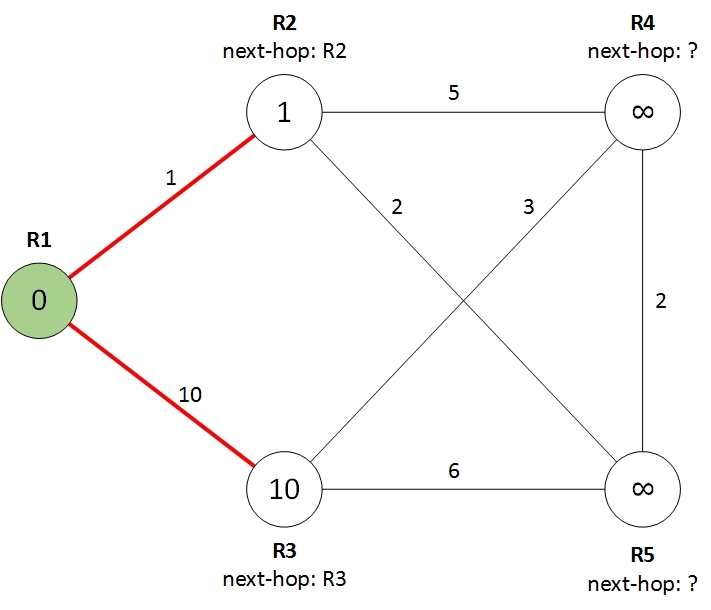
To find the shortest path, Dijkstra's algorithm is used, whose work will be considered in the following example. We have five routers interconnected by links, as shown in the figure:
')

R1 is the root router that runs the shortest path algorithm. The numbers on the links show the cost (cost) of the link. The task is to find the shortest path from router R1 to each of the other routers, i.e. the way at which the total cost of links is minimal.
As a result, for each router we need to calculate two things:
This information is necessary for R1 to correctly compile the routing table. Inside each router we will indicate the current cost to it. Next we will indicate the current next-hop that R1 uses to reach this router. Green will mark the routers to which the shortest path is calculated.
Thus, at the initial stage, we have the shortest path only to the router R1 itself, equal to 0. To the other routers, the values are infinite, and the next-hop are unknown.
Now we will take a sequence of steps, each of which will improve the cost of the paths to the routers, and ultimately we will calculate the shortest paths to all of them.
The neighbors of the root router R1 are the routers R2 and R3. For each of them, we set the cost of the path equal to the cost of the corresponding link and the next-hop is equal to the R2 or R3 router itself, as shown in the figure:
At this step, we look at all the remaining routers, i.e. routers to which the shortest path has not yet been found (white) and choose from them the router with the lowest cost of the path to it. In our case, this is R2 router with a cost of 1. We can safely repaint this router in green, there is no shorter way for it.

In the figure, it is painted in a darker green color, since this router will come in handy in step 3.
This step is similar to step 1, but instead of R1, we are looking at the neighbors of the dark green router selected in the previous step. For each neighbor, we calculate the cost of the path through the selected router. If the cost of such a path is less than the current value, then we assign a new cost to the neighbor, and simply copy the next-hop from the selected router. It turns out this picture:

Now repeat steps 2 and 3 until all routers turn green. At stage 2, we have one router necessarily turns green, so that this process will end sooner or later.
So, choose the best of the remaining ones, repaint green (router R5):

We look at the neighbors of the selected router, improve the cost, copy the next-hop:

It can be seen that R3 has changed next-hop, which was copied from R5. Choose the best:
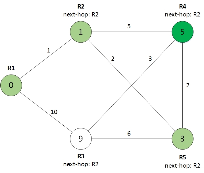
We look at the remaining neighbor:

And we get the final result:

Now we have the cost of the paths to each of the routers, as well as which next-hop to use on the root router to achieve them. Those. we are almost ready to create a routing table. However, for direct application in networks, the above algorithm requires some modernization.
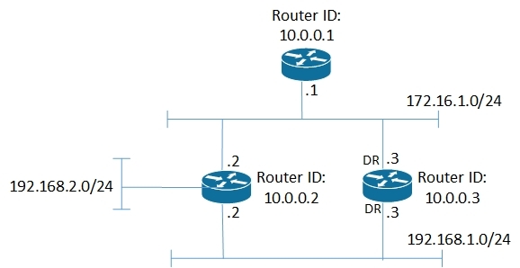
The above algorithm works only with point-to-point links, when each link connects two routers. Real routers can be connected to each other via an Ethernet network that allows more than 2 routers to connect to one segment, as shown in the figure.
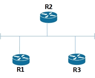
In the OSPF protocol, such a network is called transit. To solve this problem in OSPF, each transit network is represented by a separate node in the graph. Those. when calculating the shortest path, the topology will look like this:

Node N1 is just the transit network. Now we have each link connects only two nodes, and we can apply the shortest path algorithm. When calculating the cost of the path, only the cost of the link from the router to the transit network is taken into account, and from the transit network to the router it is considered equal to 0.
Since the transit network is a logical entity, one of the routers should take the responsibility to create the necessary topological information describing the transit network. To do this, in OSPF, in each transit network, a Designated Router (DR) is selected, which, in addition to information about itself, also has the obligation to announce information about the transit network.
In addition, in the routing table there are routes not to routers, but to ip networks. The issue with transit networks is solved simply. Since transit networks are represented by vertices in the graph, the cost of routes to transit networks is calculated during the operation of the shortest path search algorithm. Other networks, for example, networks to which only one OSPF router is connected, are considered final (stub) networks and are advertised by the routers to which they are connected. Knowing the cost of the shortest path to each router, you can easily calculate the cost of the route to all end networks connected to it.
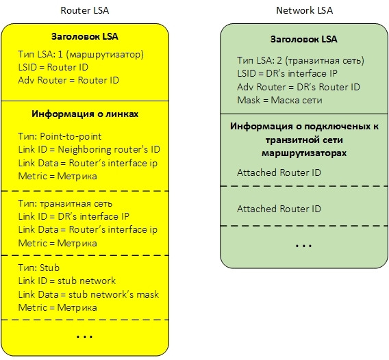
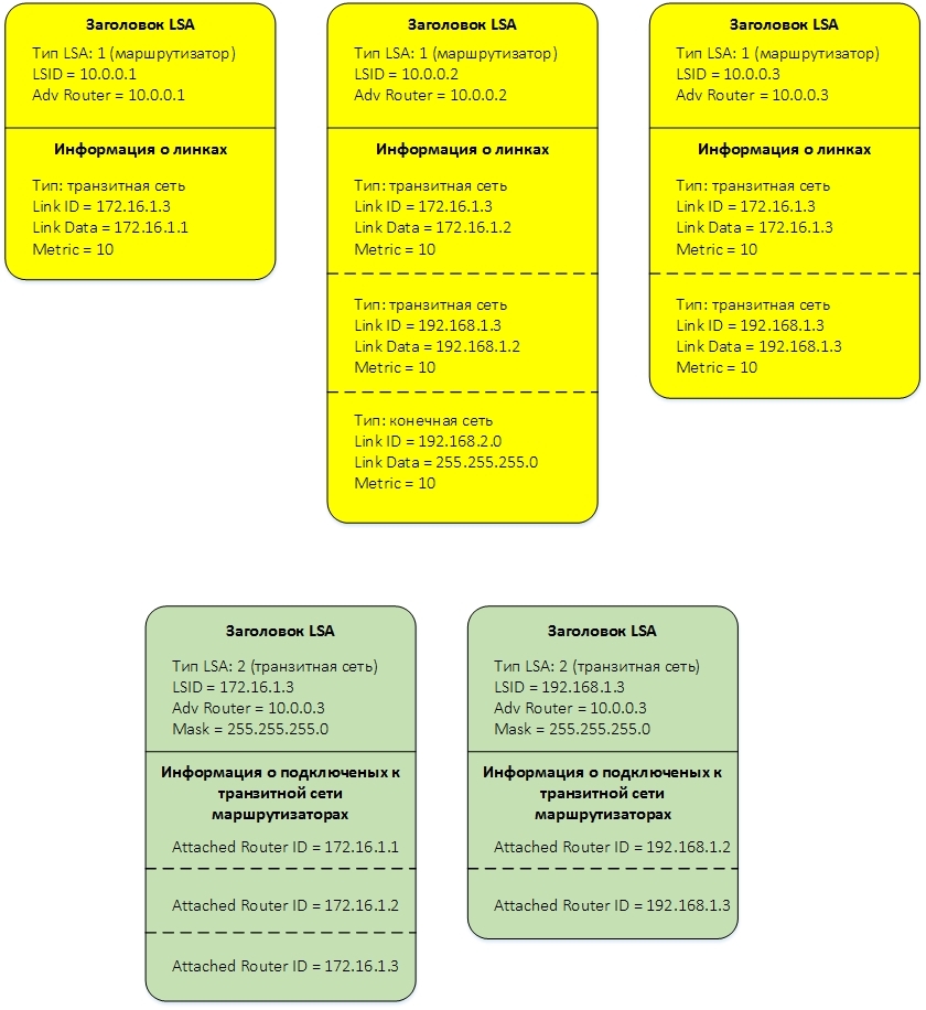
As I said, in order for each router to create a network topology and apply the shortest path search algorithm to it, the routers exchange small pieces of information with each other, called Link State Advertisement LSA. LSA come in different types and convey different information. For our case with a single zone, two types of LSA are important - LSA type 1 and LSA type 2. Each LSA type 1 describes a router. LSA type 2 describes the transit network. If we omit the various service information, then these LSA can be schematically represented as follows:
Below is a brief description of the LSA fields.
In the LSA header, we need three fields:
Below is information about the links of our router. Information about the link depends on the type of link. A router can have links of three different types:
Transit network. For a link of this type, the following information is transmitted:
Point to point. For a point-to-point link, it is transmitted:
The ultimate (stub) network. For her transmitted:
The LSA type 2 transmits the transit network information and is advertised specifically selected for each Designated Router network.
The LSA header contains four important fields:
Next comes the information about routers connected to the transit network. For each such router, its Router ID is indicated.
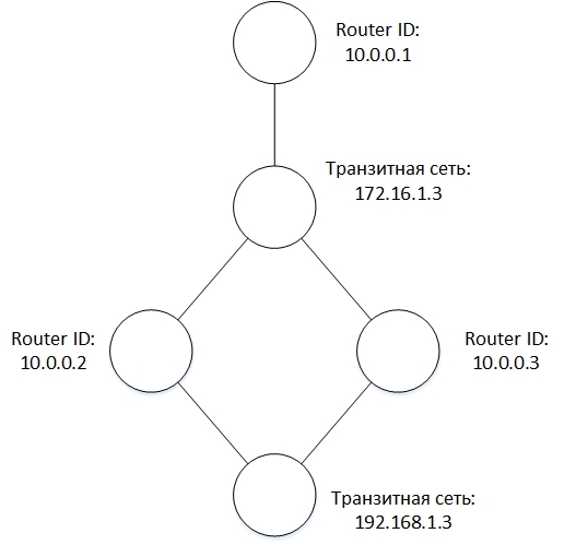
Each LSA corresponds to a graph node and, depending on the type, represents either a router or a transit network. Having all the LSA is now easy to create a network topology. For this, it is sufficient to note that the Link ID of the transit link of the router corresponds to the LSID of the transit network, and vice versa, the Attached Router ID of the transit network corresponds to the LSID of the router connected to the transit network.
For example, the figure shows a small network:
corresponding to her LSA:
and topology:
All created and received LSAs are stored in a database called LSDB (LSA Database). The main thing that is needed from this database is to be able to add LSAs to it, iterate over all LSAs of a particular type and search for LSAs by key fields from the LSA header.
You can view a list of all LSAs in LSDB and their fields using the show ip ospf database commands (displays all LSA headers), show ip ospf database route (displays full information on LSA type Router) and show ip ospf database network (displays full information on LSA network type).
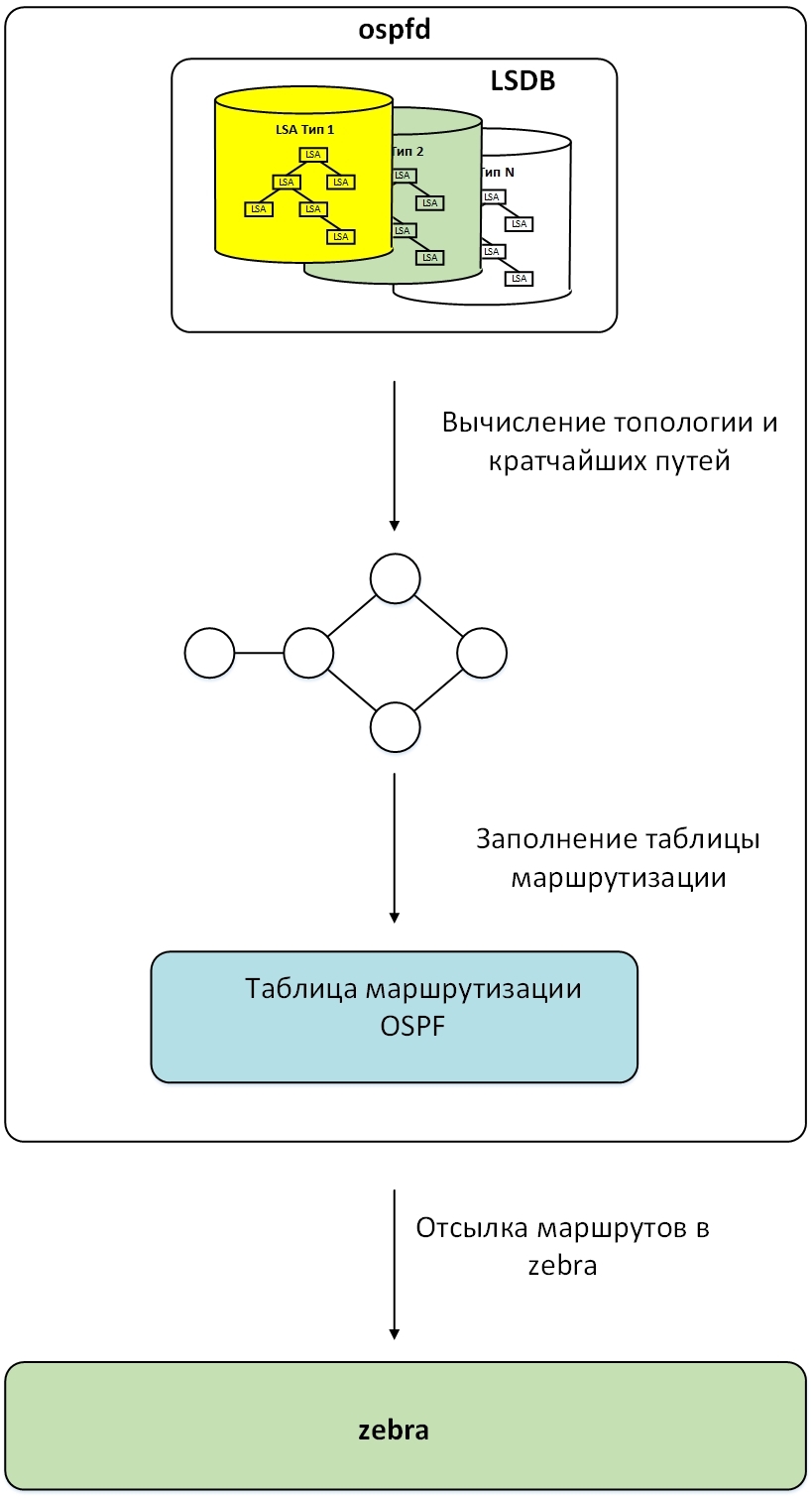
In Quagga, the entire LSA storage base (LSDB) is split into several bases, separate for each type of LSA, as shown in the figure:

Each base for storing a separate type of LSA is arranged in the same way and stores the LSAs contained in it in the form of a prefix tree described in the previous article . The prefix is a combination of LSID and Adv Router. The combination of these fields is unique for each LSA of a particular type within a zone.
When a new LSA is received, this LSA is added to LSDB and the computation of the shortest route starts. The process begins with an LSA corresponding to the router itself. Based on the information contained in it, a new node is created in memory corresponding to the root node in the topology. Next, LSDBs sequentially derive LSA, corresponding to the neighboring nodes in the topology, create new nodes and calculate the shortest paths and the next-hop to them, as described in the shortest path algorithm. In parallel, for the processed nodes, routes to transit networks are added to the OSPF routing table.
After the topology has been built and the shortest paths have been calculated, all nodes corresponding to the routers are viewed, and all their final (stub) networks are added to the OSPF routing table. Routes to transit networks have already been added to the routing table.
In the final step, all nodes in the topology are removed from memory, and routes from the OSPF routing table are transferred to the zebra daemon. The scheme of this process is shown in the figure.
As usual, I will not describe in detail the operation and configuration of the OSPF protocol, and I will refer to you where you can read more about it. I will confine myself only to the most important information for further understanding of the article.
Unlike the RIP or BGP protocols, which compare incoming routes from different neighbors and select the best ones according to some criteria, the OSPF protocol builds a topological map of the network and routes the shortest routes to the corresponding ip networks. To gather information about the network topology, routers exchange among themselves pieces of information about directly connected networks and their OSPF neighbors. These pieces of topological information are called LSA (Link State Advertisement) and from them, like a puzzle, you can assemble a complete topological map of the network. How are the LSA, we will look at later, but now we turn to the algorithm for finding the shortest path.
Algorithm for finding the shortest path
To find the shortest path, Dijkstra's algorithm is used, whose work will be considered in the following example. We have five routers interconnected by links, as shown in the figure:
')
R1 is the root router that runs the shortest path algorithm. The numbers on the links show the cost (cost) of the link. The task is to find the shortest path from router R1 to each of the other routers, i.e. the way at which the total cost of links is minimal.
As a result, for each router we need to calculate two things:
- The cost of the path from R1 to this router.
- Which next-hop uses R1 to reach this router.
This information is necessary for R1 to correctly compile the routing table. Inside each router we will indicate the current cost to it. Next we will indicate the current next-hop that R1 uses to reach this router. Green will mark the routers to which the shortest path is calculated.
Thus, at the initial stage, we have the shortest path only to the router R1 itself, equal to 0. To the other routers, the values are infinite, and the next-hop are unknown.
Now we will take a sequence of steps, each of which will improve the cost of the paths to the routers, and ultimately we will calculate the shortest paths to all of them.
Step 1. Look at the neighbors of the root router.
The neighbors of the root router R1 are the routers R2 and R3. For each of them, we set the cost of the path equal to the cost of the corresponding link and the next-hop is equal to the R2 or R3 router itself, as shown in the figure:
Step 2. Choose the best of the remaining.
At this step, we look at all the remaining routers, i.e. routers to which the shortest path has not yet been found (white) and choose from them the router with the lowest cost of the path to it. In our case, this is R2 router with a cost of 1. We can safely repaint this router in green, there is no shorter way for it.
In the figure, it is painted in a darker green color, since this router will come in handy in step 3.
Step 3. We look at the neighbors of the selected router.
This step is similar to step 1, but instead of R1, we are looking at the neighbors of the dark green router selected in the previous step. For each neighbor, we calculate the cost of the path through the selected router. If the cost of such a path is less than the current value, then we assign a new cost to the neighbor, and simply copy the next-hop from the selected router. It turns out this picture:
Now repeat steps 2 and 3 until all routers turn green. At stage 2, we have one router necessarily turns green, so that this process will end sooner or later.
So, choose the best of the remaining ones, repaint green (router R5):
We look at the neighbors of the selected router, improve the cost, copy the next-hop:
It can be seen that R3 has changed next-hop, which was copied from R5. Choose the best:
We look at the remaining neighbor:
And we get the final result:
Now we have the cost of the paths to each of the routers, as well as which next-hop to use on the root router to achieve them. Those. we are almost ready to create a routing table. However, for direct application in networks, the above algorithm requires some modernization.
Shortest Path Algorithm Update
The above algorithm works only with point-to-point links, when each link connects two routers. Real routers can be connected to each other via an Ethernet network that allows more than 2 routers to connect to one segment, as shown in the figure.
In the OSPF protocol, such a network is called transit. To solve this problem in OSPF, each transit network is represented by a separate node in the graph. Those. when calculating the shortest path, the topology will look like this:
Node N1 is just the transit network. Now we have each link connects only two nodes, and we can apply the shortest path algorithm. When calculating the cost of the path, only the cost of the link from the router to the transit network is taken into account, and from the transit network to the router it is considered equal to 0.
Since the transit network is a logical entity, one of the routers should take the responsibility to create the necessary topological information describing the transit network. To do this, in OSPF, in each transit network, a Designated Router (DR) is selected, which, in addition to information about itself, also has the obligation to announce information about the transit network.
In addition, in the routing table there are routes not to routers, but to ip networks. The issue with transit networks is solved simply. Since transit networks are represented by vertices in the graph, the cost of routes to transit networks is calculated during the operation of the shortest path search algorithm. Other networks, for example, networks to which only one OSPF router is connected, are considered final (stub) networks and are advertised by the routers to which they are connected. Knowing the cost of the shortest path to each router, you can easily calculate the cost of the route to all end networks connected to it.
Link State Advertisement (LSA)
As I said, in order for each router to create a network topology and apply the shortest path search algorithm to it, the routers exchange small pieces of information with each other, called Link State Advertisement LSA. LSA come in different types and convey different information. For our case with a single zone, two types of LSA are important - LSA type 1 and LSA type 2. Each LSA type 1 describes a router. LSA type 2 describes the transit network. If we omit the various service information, then these LSA can be schematically represented as follows:
Below is a brief description of the LSA fields.
LSA Type 1 (Router LSA).
In the LSA header, we need three fields:
- Type of. Indicates the type of LSA. In our case, this is type 1, or Router LSA.
- LSID. LSA ID. In our case, the LSID is equal to the Router ID of the router that creates the LSA.
- Adv Router. ID of the router that created the LSA. In our case, it is also equal to the Router ID of the router that creates the LSA, i.e. matches the LSID.
Below is information about the links of our router. Information about the link depends on the type of link. A router can have links of three different types:
Transit network. For a link of this type, the following information is transmitted:
- Link ID - ip-address of the Designated Router interface connected to the transit network.
- Link Data - ip-address of the interface of the router itself connected to the transit network.
- Metric - link cost.
Point to point. For a point-to-point link, it is transmitted:
- Link ID - ip-address of the neighbor interface.
- Link Data - ip-address of the interface of the router itself.
- Metric - link cost.
The ultimate (stub) network. For her transmitted:
- Link ID - the actual IP address of the network.
- Link Data - network mask.
- Metric - link cost.
LSA Type 2 (Network LSA)
The LSA type 2 transmits the transit network information and is advertised specifically selected for each Designated Router network.
The LSA header contains four important fields:
- Type of. In our case, this is type 2, or Network LSA.
- LSID. LSA ID. In our case, the LSID is equal to the ip-address of the Designated Router interface connected to the transit network;
- Adv Router. ID of the router that created the LSA. In our case, it is equal to Designated Router ID.
- Mask. Net mask
Next comes the information about routers connected to the transit network. For each such router, its Router ID is indicated.
Each LSA corresponds to a graph node and, depending on the type, represents either a router or a transit network. Having all the LSA is now easy to create a network topology. For this, it is sufficient to note that the Link ID of the transit link of the router corresponds to the LSID of the transit network, and vice versa, the Attached Router ID of the transit network corresponds to the LSID of the router connected to the transit network.
For example, the figure shows a small network:
corresponding to her LSA:
and topology:
All created and received LSAs are stored in a database called LSDB (LSA Database). The main thing that is needed from this database is to be able to add LSAs to it, iterate over all LSAs of a particular type and search for LSAs by key fields from the LSA header.
You can view a list of all LSAs in LSDB and their fields using the show ip ospf database commands (displays all LSA headers), show ip ospf database route (displays full information on LSA type Router) and show ip ospf database network (displays full information on LSA network type).
Implementation in Quagga
In Quagga, the entire LSA storage base (LSDB) is split into several bases, separate for each type of LSA, as shown in the figure:
Each base for storing a separate type of LSA is arranged in the same way and stores the LSAs contained in it in the form of a prefix tree described in the previous article . The prefix is a combination of LSID and Adv Router. The combination of these fields is unique for each LSA of a particular type within a zone.
When a new LSA is received, this LSA is added to LSDB and the computation of the shortest route starts. The process begins with an LSA corresponding to the router itself. Based on the information contained in it, a new node is created in memory corresponding to the root node in the topology. Next, LSDBs sequentially derive LSA, corresponding to the neighboring nodes in the topology, create new nodes and calculate the shortest paths and the next-hop to them, as described in the shortest path algorithm. In parallel, for the processed nodes, routes to transit networks are added to the OSPF routing table.
After the topology has been built and the shortest paths have been calculated, all nodes corresponding to the routers are viewed, and all their final (stub) networks are added to the OSPF routing table. Routes to transit networks have already been added to the routing table.
In the final step, all nodes in the topology are removed from memory, and routes from the OSPF routing table are transferred to the zebra daemon. The scheme of this process is shown in the figure.
Source: https://habr.com/ru/post/316518/
All Articles