Low-level optimization and measurement of code performance on R

Over the past decade, R has come a long way: from the niche (as a rule, academic) tool to the mainstream “big ten” most popular programming languages. Such interest is caused by many reasons, among which are membership in open source, an active community, and an actively growing segment of the application of machine learning / data mining methods in a variety of business tasks. It's nice to see when one of your favorite languages ​​confidently gains new positions, and when even users who are far from professional development become interested in R. But there is, however, one big problem: R language is written, in the words of the creators, "statisticians for statisticians." Therefore, it is high-level, flexible, with a huge and reliable functionality out of the box, not to mention thousands of additional packages; and at the same time, it is a very frivolous in terms of semantics, combining fundamentally different paradigms and possessing wide possibilities for writing monstrously inefficient code. And if we take into account the fact that lately this is the first "real" programming language for many, the situation becomes even more threatening.

However, improving the quality and speed of code execution on R is a universal task that not only beginners, but also experienced users constantly face. That is why it is very important to return from time to time to the simplest structures and basic principles of R work, in order to remember the sources of inefficiencies and ways to eliminate them. In this article I will talk about one case that I first met during the work on the study of financial strategies, and then was adapted by me as a training course for an online course.

How not to get caught in the matrix

Omitting all irrelevant details, we can formulate our test problem as follows. For arbitrary natural you need to quickly generate matrices of size of this kind (an example is given for ):

1 2 3 4 5 2 3 4 5 4 3 4 5 4 3 4 5 4 3 2 5 4 3 2 1 

This is a special case of the so-called Hankel matrices . Here, the upper left and lower right corners always contain one, the entire secondary diagonal (from the lower left to the upper right corner) consists of the number , and all other values ​​are located by steps. As a result, we have something similar to a mountain range or roof slope.

It is natural to expect that the parameter can vary in some reasonable range, say, from units to hundreds. Therefore, we will solve the problem as a separate function, and will be an argument in it.

The simplest calculation shows that the matrix we need is determined elementwise using the condition . If we wrote in one of the classical imperative languages ​​(such as C or C ++ ), then the solution would be complete, since it reduces to an elementary double loop. On R, this “naive solution” looks like this:

 build_naive <- function(n) { m <- matrix(0, n, n) for (i in 1:n) for (j in 1:n) m[i, j] <- min(i + j - 1, 2*n - i - j + 1) m } 

Even in spite of the fact that we initialize the matrix of the required size in advance (the absence of the first row — preallocation of memory — a frequent error of beginners), this solution works very slowly. For experts on the language, such a result is quite predictable: since R is an interpreted language, each iteration of the cycle entails a lot of overhead for execution. Examples with non-optimal use of cycles are found, perhaps, in every textbook on R. And the conclusion is always the same: if possible, use the so-called vectorized functions. They are usually implemented at a low level (C) and extremely optimized.

So, in our case, when the matrix element is a function of two indices and , a combination of the outer and pmin functions pmin :

 build_outer_pmin <- function(n) { outer(1:n, 1:n, function(i, j) pmin(i + j - 1, 2*n - i - j + 1)) } 

The pmin function differs from min in that it operates with vectors on both the input and the output. Compare: min(3:0, 1:4) searches for a common minimum (zero in this case), and pmin(3:0, 1:4) returns a vector from pairwise minima: (1, 2, 1, 0) . The concept of vectorized function is not easy to formulate formally, but the general idea, I hope, is understandable. This is the function that the outer function expects as an argument. That is why it is impossible to pass min into it, as in a naive solution, try this and make sure that an error occurs. By the way, if we still want to use a combination of outer and min , we can perform a forced vectorization of the min function, wrapping it in the Vectorize function:

 build_outer_min <- function(n) { outer(1:n, 1:n, Vectorize(function(i, j) min(i + j - 1, 2*n - i - j + 1))) } 

It should be remembered at the same time that compulsory vectorization of this kind will always work more slowly than the natural one. However, in some situations it is Vectorize to do without Vectorize - for example, if the definition of a matrix element contains a conditional if .

Another way to get rid of the inefficiency of a naive solution is to somehow remove the nesting of cycles — it is to iterate not by the unit elements of the matrix, but by the vectors or submatrices. There can be many options, I will show only one of them, recursive. We will build the matrix "by the floor", from the center to the edges:

 build_recursive <- function(n) { if (n == 0) return(0) m <- matrix(0, n, n) m[-1, -n] <- build4(n - 1) + 1 m[1, ] <- 1:n m[, n] <- n:1 m } 

In this case, efficiency is achieved due to the fact that the number of high-level iterations is not , as in a naive decision, but only (the role of the loop is taken by the call stack).

Finally, in the case when optimization at the level of basic functions R does not lead to the desired result, there is always another option: implement the slow part at the lowest possible level. That is, to write a piece of code in pure C or C ++, compile it and call it from R. Such an approach is popular among package developers because of its extreme efficiency and simplicity, and also because there is a great Rcpp package for working with C ++ .

 library(Rcpp) cppFunction("NumericMatrix build_cpp(const int n) { NumericMatrix x(n, n); for (int i=0; i<n; i++) for (int j=0; j<n; j++) x(i, j) = std::min(i + j + 1, 2*n - i - j - 1); return x;}") 

When we call cppFunction in a similar way, the code will be compiled in C ++ , and upon its completion we will get the build_cpp function in the global environment, which can be called like any other function we have defined. Of the obvious drawbacks of such an approach, the need to compile can be noted (this also takes time), not to mention the fact that it is necessary to be fluent in C ++ . Of course, using Rcpp not a “silver bullet”, and writing slow C / C ++ code is also quite simple.

microbenchmark package

When we talked about the speed of decisions, we relied on a priori knowledge of how language works. Theory is theory, but any reasoning about performance should be accompanied by experiments - measuring the time of execution with specific examples. Moreover, in such cases it is always better to check and recheck everything yourself, because any such measurements are not absolute truth: they depend on the hardware and the state of the processor, on the operating system and its load at the time of measurement.

There are several typical ways to measure the speed of code execution on R. One of the most common is the system.time function. When using this function, they usually do something like system.time(replicate(expr, 100)) . This is a good option, but there are several packages that do the same, but in a much more convenient and customizable version. In fact, the standard is a package called microbenchmark , which we will use. All work will be performed by a function of the same name, to which you can pass an arbitrary number of expressions (see unevaluated expression ) for measurement. By default, each expression will be executed a hundred times, and we will see the collected statistics on the execution time.

 library(microbenchmark) measure <- function(n) { microbenchmark(build_naive(n), build_outer_min(n), build_outer_pmin(n), build_recursive(n), build_cpp(n)) } m <- measure(100) m Unit: microseconds expr min lq mean median uq max neval build_naive(n) 20603.310 21825.7975 24380.0332 22884.3255 24215.368 66753.031 100 build_outer_min(n) 22624.873 25430.4985 28164.4496 26662.8955 29028.744 84972.926 100 build_outer_pmin(n) 159.755 187.8325 295.3822 204.1985 225.069 3710.103 100 build_recursive(n) 1741.992 2822.2910 5990.9897 3241.1980 3918.055 55059.974 100 build_cpp(n) 21.321 23.4230 33.6600 34.2335 38.588 91.289 100 

In the obtained output, the measurement results are presented in the form of a table with a set of descriptive statistics. In addition, the resulting object can be drawn: plot(m) or ggplot2::autoplot(m) .

Package benchr

Currently, another package is being developed, designed to measure the execution time of expressions - the benchr package. The functionality and syntax is almost identical to the microbenchmark package, but with some key differences. Briefly, these differences can be described as follows:

1. We use a single cross-platform measurement mechanism based on a timer from C ++ 11;
2. The user is provided with more options to configure the measurement process;
3. The output of text and graphic results becomes more detailed and visual.

The benhcr package is in CRAN (for version R older than 3.3.2), and the development version is available on gitlab , there are also installation instructions. Using benchr in our example will look like this (all you need is to replace the microbenchmark function with the benchmark function):

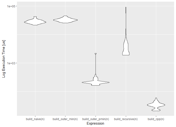
 install.packages("benchr") library(benchr) measure2 <- function(n) { benchmark(build_naive(n), build_outer_min(n), build_outer_pmin(n), build_recursive(n), build_cpp(n)) } m2 <- measure2(100) m2 Benchmark summary: Time units : microseconds expr n.eval min lw.qu median mean up.qu max total relative build(n) 100 21800 24300 25600.0 27400.0 28100.0 79300.0 2740000 906.00 build2(n) 100 24400 28800 30100.0 31600.0 33700.0 44000.0 3160000 1070.00 build3(n) 100 157 189 198.0 738.0 217.0 43400.0 73800 7.02 build4(n) 100 1820 1980 3380.0 4910.0 4050.0 50000.0 491000 120.00 build5(n) 100 21 27 28.2 29.4 30.5 50.1 2940 1.00 

In addition to convenient textual output (the relative column allows you to quickly evaluate the advantage of the fastest solution), we can use various visualizations. By the way, if you have the ggplot2 package ggplot2 , it will be used for drawing graphs. If for some reason you do not want to use ggplot2 , this behavior can be changed using the benchr package benchr . Three typical visualization of the measurement results are now supported: dotplot, boxplot and violin plot.

 plot(m2) boxplot(m2) boxplot(m2, violin = TRUE)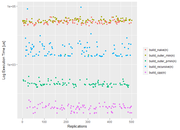 

Results

So, according to the results of measurements, we can formulate the following conclusions.

1. The reference (naive) solution works slowly, since a double for loop produces high-level iterations, which does not correspond to the vectorial orientation of the language R;
2. Direct transfer of the loop to the outer function with forced vectorization via Vectorize does not solve the problem, because the solution is semantically identical to the naive one;
3. The recursive solution is faster by an order of magnitude, because high-level iterations become , and operations with submatrices in R are fast enough;
4. Using outer in combination with the natural vectorization of the pmin function is two orders of magnitude faster due to the low-level implementation (compiled C);
5. Direct access to Rcpp is three orders of magnitude faster (without taking into account C ++ compilation time), since the Rcpp package Rcpp additionally optimized with the help of modern features of the C ++ language.

And now the most important thing that I would like to bring this article. If you know how the language of R and what philosophy he professes; if you remember about the natural vectorization and a powerful set of functions of the base R; Finally, if you arm yourself with modern means of measuring the execution time, then even the most difficult task can turn out to be quite lifting, and you will not have to spend long minutes and even hours waiting for the completion of your code.

Small disclaimer: the benchr package benchr conceived and implemented by Artem Klevtsov ( @artemklevtsov ) with additions and improvements from me (Anton Antonov, @tonytonov ) and Phillip Upravitelev ( @konhis ). We will welcome bug reports and feature suggestions.

Tasks like this form the basis of the course “Basics of Programming on R” on the Stepik.org platform. The course is open without deadlines (it can be held at a free pace) and is included in the data analysis professional retraining program (SPbAU RAS, Institute of Bioinformatics ).

If you are in St. Petersburg, we will be glad to see you at one of the regular meetings of the SPb R user group ( VK , meetup ).

Materials and additional reading on the topic:

1. Norman Matloff, The Art of R Programming: A Tour of Statistical Software Design
2. Patrick Burns, The R Inferno
3. Hadley Wickham, Advanced R
4. Dirk Eddelbuettel, Seamless R and C ++ Integration with Rcpp
5. A. B. Shipunov, E. M. Baldin et al. Visual statistics. Use R!