Generation and selection of machine learning models. Lecture in Yandex
The use of machine learning can include working with data, fine-tuning an already trained algorithm, etc. But a large-scale mathematical preparation is also needed at an earlier stage: when you only choose a model for further use. You can choose "manually" using different models, but you can also try to automate this process.
Under the cut - a lecture by leading researcher of the Russian Academy of Sciences, doctor of science and editor-in-chief of the Machine Learning and Data Analysis journal Vadim Strizhov, as well as most of the slides.
We will talk about ways of generating and selecting models using the example of the time series of the Internet of things.
')
The concept of the Internet of things appeared more than ten years ago. From the usual Internet, it differs primarily in the fact that the request is not made by a person, but by a device or message on a network that interacts with other devices without a person.
The first example. No one wants to climb into the corner with a flashlight every month, look at how much the electricity meter is wrapped around, and then go up and pay. It is clear that modern meters monitor not only hourly energy consumption in an apartment, but even know how much energy has been taken from each outlet.
The second option. Monitoring human health. An example of time series that are in this area is the following. Now patients with tetraplegia, whose limbs have failed, put a palm-sized sensor directly on the cortex. It is not visible from the inside, it is completely closed. It gives 124 channels from the surface of the cortex with a frequency of 900 hertz. In these time series, we can predict the movement of limbs, the way he wants to move.
The next example is trading. Now cashiers exit the store are expensive, and the queue at the exit of the store is not good either. It is required to create such a system and receive such signals when a person with a cart, driving past the exit, immediately receives all the price values of the products he purchased.
The last rather obvious example is the automatic regulation of the work of urban services: traffic lights, lighting, weather sensors, floods, etc.

Here is the first example of a time series with which we will work. We have hourly electricity consumption, maximum and minimum daily temperature, humidity, wind, day length.

The second example of time series, which is hierarchically located above the first, is the same, only for each point of a certain region. In this case, a piece of Europe is shown, and together with these time series, in particular, the value of air pollution is removed at each point.

An even more complex example is the values of the electric field. Frequencies are plotted along the ordinate axis, time is plotted along the abscissa. This is also a time series. If the last time series is the Cartesian product of time and space into space, here we have the Cartesian product of time and frequencies.
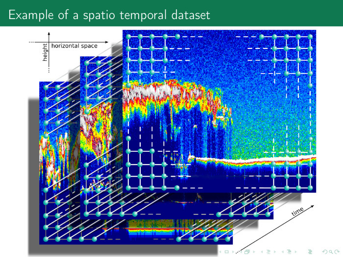
The next time series is even more complex. The axis of abscissa and ordinate space, on the axis of applicat - time. Thus, we have many different beautiful time series, and the time series does not necessarily contain only time and values. It may contain a Cartesian product of several time axes, frequencies, spaces, etc.
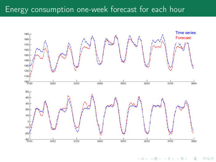
Consider the easiest option. We have time series of electricity consumption of a small city. There is a price, volume of consumption, day length, temperature, etc. These time series are periodic. Electricity consumption fluctuates during the year, during the week and during the day.
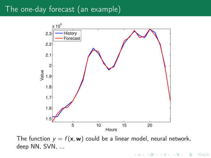
Take an arbitrary day. Blue - time series, red - forecast. 12 at night, citizens fall asleep, the mafia wakes up. The time series falls, consumption falls. All of Moscow is lit at night with lights, in general, because it is surrounded by CHP, there is nowhere to put the energy, and the price of electricity may even fall below zero, and you can pay extra for electricity - just to consume.
6 hours, citizens wake up, go to work, drink tea, then work, then go home - this cycle repeats.
The task is to forecast the electricity consumption by the next day by the hour and purchase all the electricity for a day at once. Otherwise, the next day will have to pay extra for the difference in consumption, and this is more expensive.
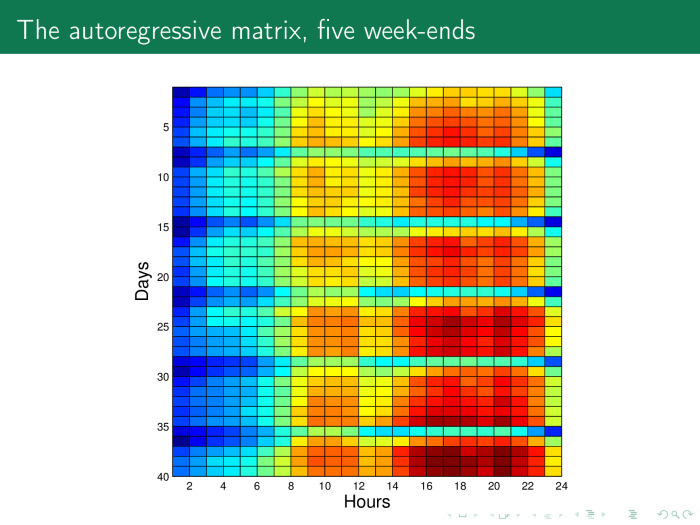
How is this problem solved? Let's build such a matrix based on the previous time series. Here in rows are days, about 40 days for 24 hours. And we can easily see special lines here - Saturdays and Sundays. It can be seen that in Ankara, as well as in Moscow, on Saturday people behave quite actively, and rest on Sunday.
Each column - in this case 20 hours of a day of the week. There are five weeks in total.

Imagine this matrix in formal form. We take the time series by the tail, by days of the week or by weeks we turn, we get an object – feature matrix, where the object is the day, and the sign is an hour, and we solve the standard linear regression problem.
Using this value, we are looking for, for example, 12 o'clock the next day. What we predict, we count y for our entire history. X - the whole story, except these 12 hours. The forecast is the scalar product of the last week, the vectors of values and our weights, which we obtain, for example, using the method of least squares.
What needs to be done to get a more accurate forecast? Let's spawn the various elements of the model. We call them generating functions or primitives.

You can do the following with the time series: take the root from it. You can leave it, you can take the time series - the root of the time series, the time series - the logarithm of the time series, etc.
Thus, we add columns to the matrix object – feature, increase the number of columns, and the number of rows remains the same.
Moreover, we can use the Kolmogorov-Gabor polynomial to generate features. The first member is the time series itself. The second member is all the works of time series. The third is the product of time series triples. And so on, until we get bored.
The coefficient is collected from the entire time series - and again we obtain a linear model. After that we get a pretty decent forecast. And even there is a suspicion whether we have not retrained, is the forecast too good?
He is just as good that the parameters have generally lost their meaning.
Suppose the row of matrices of the plan is a week, 7 days, 168 hours. There are data, for example, for three years. There are 52 weeks in the year. Then the three-year base matrix is 156 rows by 168 columns.
If we use six time series that I will list, that is, together with the consumption, we also take into account price, humidity, temperature, and so on, then there will be more than 1000 columns in the matrix. And if there are four more generating functions, then these are 4000 rows and 156 columns. That is, the matrix is strongly degenerate, and it is not possible to solve the linear equation normally. What to do?
Probably, you need to run the procedure for selecting models. To do this, look at what weights make sense. For each hour we build our model, and here on the x-axis shows the values of the model parameters by the hour on the next day. And on the y-axis are the parameters themselves. We see a yellow-red diagonal, the value of the scales is larger where there is an hour in the model for the previous days.
The principle is simple. The forecast for tomorrow at 12 o'clock depends on the values for 12 hours of the previous day, the day before yesterday, and so on. Thus, we can leave only these values and throw away everything else.
What exactly should be discarded? Imagine the matrix x as a set of columns. We approximate the time series y with a linear — or optionally linear — combination of columns of the matrix x. We would like to find a column χ that would be closer to y. A significant part of the feature selection algorithms will select the columns χ 1 and χ 2 if we want to leave two columns. But among those that we have created, we need χ 3 and χ 4 . They provide both an accurate and stable model. Exact - because the linear combination of χ 3 and χ 4 exactly approximates y, and stable - because they are orthogonal.
Why two columns? We need to see in which space we are working, how many objects are in the drawn sample. Here are three objects. Matrix x contains 3 rows and 6 columns.
How do feature selection algorithms work? As a rule, they use error functions. In linear regression, this is the sum of the squares of the regression residuals. And there are two types of feature selection algorithms. The first type is regularizing algorithms. In addition to error, they use, as was said by Konstantin Vyacheslavovich in the last lecture, also some regularizer, a penalty on the value of the parameters and some coefficient, which is responsible for the importance of the penalty.
This coefficient can be represented in the form of such or such a fine. The weights must be no more than some value of τ.
In the first case, it is not about the loss of the number of columns in the matrix x, the number of features, but only about increasing stability. In the second case, we just lose a significant number of columns.
It is important to understand how the columns correlate with each other. How to find out?
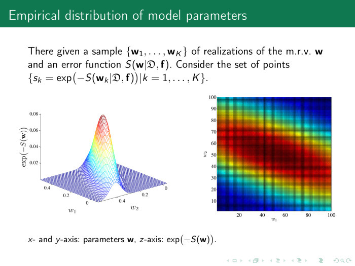
Consider the parameter space of our model, the vector w, and calculate the value of the error at various points of w. The picture on the right shows the space itself, w 1 or w 2 . Two weights are sampled, 100 points each. It turns out 100 pairs of scales. Each point of this figure is the value of the error function. On the left, for convenience, the same is the exponent of the minus value of the error function.
It is clear that the optimal values lie somewhere in the point of 0.2–0.25 and this is what we are looking for. And the importance of the parameters is defined as follows: let's take a little bit of the parameter values from the optimal value. If we change w, the error function practically does not change. Why do we need such a parameter? Probably not needed.
Here, the value of the parameters slightly rocked along the w 2 axis, the error function dropped - fine. This basis of parameter space analysis is a way to find multi-correlating features.
Where do these signs come from? Let's look at the four main ways of generating signs. The first is the signs themselves. Where are they from? We take a time series and chop it into pieces, for example, multiples of a period. Or just by chance, or with overlap. We add these chopped segments into matrix X, the plan matrix.
The second way. Same. We transform the time series using some parametric or non-parametric features.
The third method is very interesting and promising. We are bringing pieces of the time series with some models. We will call this local modeling. And we use the parameters of these models as signs for the forecast.
Fourth. Everything happens in some kind of metric space. Let's find the centroids, cluster thickening in this space, and consider the distances from each time series to the centroids of these clusters.

Bad news. In order to build a matrix of the plan, the ratios of frequencies to sampling time series, if the series are different, should be short. In this case, the matrix of the plan grows. True, you can throw out some parts of the time series, as shown here. The entire time series “day length” is not needed, only one point per day is needed, and the plan matrix will look like this: 24 points in a row is electricity consumption, and one point and one more is the length of the daylight hours.
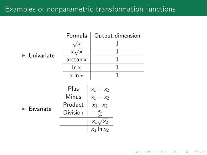
Here is the time series. What we have already reviewed. x ln x, in pairs, is the sum, difference, product, and various other combinations.

Here are non-parametric transformations. Just the average amount, the standard deviation. Histogram of time series quantiles.
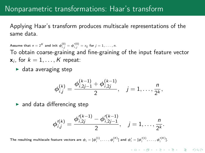
The next option. Nonparametric transformation, Haar transform. We take the arithmetic average and put it as a single point instead of two. Or take the difference. Thus, we generate the feature and reduce the number of points in the time series, respectively, reduce the dimension of space.
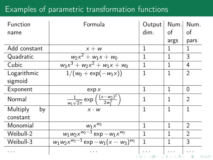
The next set of generating functions is parametric functions. With them, we can approximate the time series. The first is to use this approximate series instead of the initial one. The second is to use the parameters themselves, denoted as w.
Constant, parabola, hyperbola, logarithmic sigmoid, product, power functions, exponential functions.
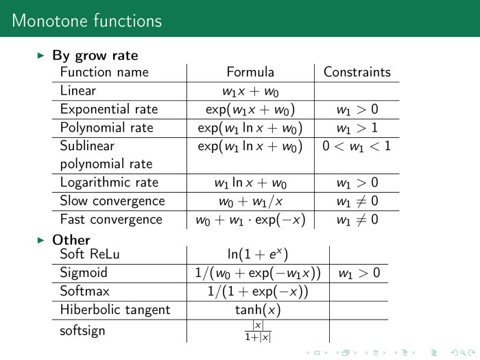
Another very convenient class is monotone functions. Here neural network experts can see, for example, activation functions that are often used in networks. They can be used not only at the output of networks, but also at the entrance. This also greatly improves the quality of the forecast.

The next class of generating functions is parametric time series transformations. Here we are interested in the parameters of the series themselves. We take the above functions and collect their parameters in the vector b. We have two types of parameters: the first is the parameters of the approximating functions themselves, local approximation functions, and the second vector are the model parameters, those that were considered earlier, that is, the weight parameters of linear combinations of columns of the X matrix. We can adjust them simultaneously, or we can set up iteratively and use them including as columns of the design matrix. In other words, the matrix of the plan, X, changes iteratively.
Where else can we get the parameters of the models? I will consider from the end. The splines in the approximation of the time series have parameters, nodes of splines.
Fast Fourier transforms. Instead of a time series, we can use its spectrum and also insert it into the matrix of the object – feature.
An important and well-working technique is to use the parameters of the “Singular structural analysis” or “Caterpillar” method.
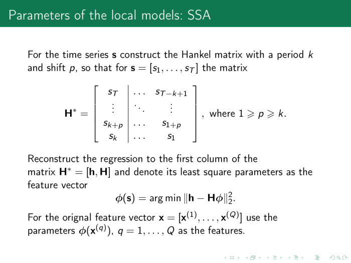
This method works as follows. First, we built the matrix X - let's build a new matrix in a similar way. Now the local approximation matrix will be called H, and it will be constructed as follows: the segment of the time series enters the rows of the matrix, not one after the other, but with overlap. Let here p = 1, and k = 3. The matrix by indices will look like 1,2,3; 2,3,4; 3,4,5 and so on to the end.
Adjust the last column of the previous we will be the same method of least squares, and the coefficients used as our signs. In particular, this technique works well in determining physical activity. For example, an athlete has a watch on his arm and an athlete wants to understand how efficiently he is moving. This task is especially popular with swimmers. It is required to determine not only the type of swim, but also the power of the stroke.
The processor is weak there, no memory. And instead of solving a large problem of determining the class of a time series or predicting a series, we immediately approximate it in a similar way when we receive data. We use not an approximated time series, but approximation parameters.
This is why it works.
It shows not the time series itself, but its logged values. This point is the value of the series at a given time and one count later. It is clear that the sine will look like an ellipse. The good news is that the dimension of this ellipse in the space of logged variables will always be 2. Whatever length of prehistory we take in this space, the dimension of the space will still remain fixed. And the dimension of space can always be determined by singular decomposition.

Then we can represent each time series in the form of its main components in a singular decomposition. Accordingly, the first main component will be some kind of trend, the second - the main harmonic and so on in ascending harmonics. We use the weights of these components as attributes in approximating models.
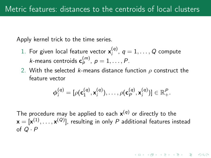
Here is the last way to generate traits. Signs are metric. We have already somehow generated the plan matrix - let's see how its columns are located in some kind of metric space, for example, in Euclidean space.
We assign the metric ρ and cluster the rows of the object – feature matrix, X.
Naturally, the number of distances from all objects in the sample to all objects in the sample is the power of the sample in the square. Therefore, we select the centers of the clusters, measure the distance from each row to the center, and use the obtained distances as signs in the matrix of the object-attribute.
In practice, it looks like this. In order for the distance to be calculated correctly, we first align the time series. It shows six classes of rows for the accelerometer: a person goes, goes up the steps, down the steps, stands and lies. It is proposed to first align the rows with a procedure and get, for example, such rows. Next - calculate the average values or centroids for each row.
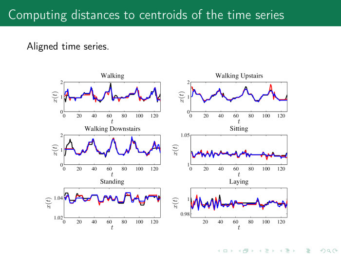
And then calculate the distance from each time series in the matrix X, the object – feature, to these centroids.
What happened as a result of generating signs in different ways? Let's look at the same data as in the beginning.
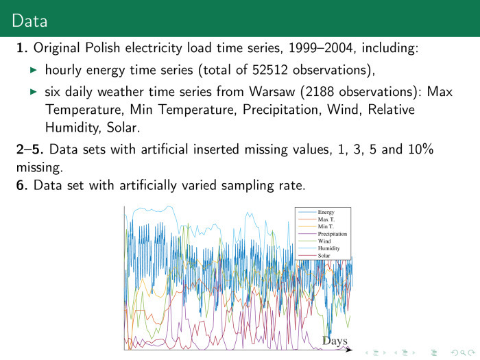
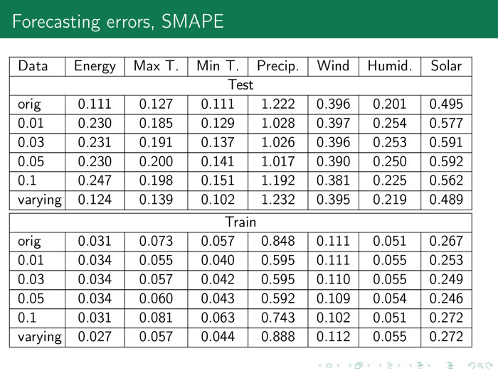
This is the data of power consumption in Poland, they are hourly. In addition, they are accompanied by different time series that describe them. We also insert gaps into this sample. Throw away some data, for example 3, 5, 10%. Fill them, and then try to predict the value of all the series at once.
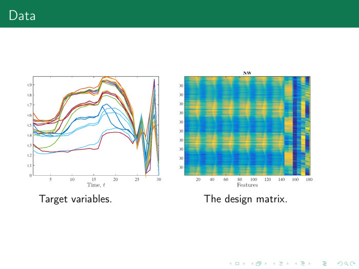
On the right, we get the following object – feature matrix. On the left, time series, chopped into pieces. The first 24 time series - day. Instead of a zigzag, you should build a histogram.

What models do we have? The best model is the forecast for tomorrow, the same as today. We will call this the base method.
Linear regression, which we considered at the beginning. Support vector machine. Neural network random forest. Of course, the fourth magic method was not enough. There are four methods that always work well, if the problem is solved at all: neural networks, support vectors, random forest and gradient boosting.
Let's compare how four different methods work with different ways of generating signs. Here again, these four ways. Historical time series. The approximation of time series. — .
. — , . — .
. . , . – , . , — . Support vector machine . random forest . .

. , support vector regression . , . , , , , . — support vector regression . , .
? , , - , . : , , - , , . , .
Under the cut - a lecture by leading researcher of the Russian Academy of Sciences, doctor of science and editor-in-chief of the Machine Learning and Data Analysis journal Vadim Strizhov, as well as most of the slides.
We will talk about ways of generating and selecting models using the example of the time series of the Internet of things.
')
The concept of the Internet of things appeared more than ten years ago. From the usual Internet, it differs primarily in the fact that the request is not made by a person, but by a device or message on a network that interacts with other devices without a person.
The first example. No one wants to climb into the corner with a flashlight every month, look at how much the electricity meter is wrapped around, and then go up and pay. It is clear that modern meters monitor not only hourly energy consumption in an apartment, but even know how much energy has been taken from each outlet.
The second option. Monitoring human health. An example of time series that are in this area is the following. Now patients with tetraplegia, whose limbs have failed, put a palm-sized sensor directly on the cortex. It is not visible from the inside, it is completely closed. It gives 124 channels from the surface of the cortex with a frequency of 900 hertz. In these time series, we can predict the movement of limbs, the way he wants to move.
The next example is trading. Now cashiers exit the store are expensive, and the queue at the exit of the store is not good either. It is required to create such a system and receive such signals when a person with a cart, driving past the exit, immediately receives all the price values of the products he purchased.
The last rather obvious example is the automatic regulation of the work of urban services: traffic lights, lighting, weather sensors, floods, etc.
Here is the first example of a time series with which we will work. We have hourly electricity consumption, maximum and minimum daily temperature, humidity, wind, day length.
The second example of time series, which is hierarchically located above the first, is the same, only for each point of a certain region. In this case, a piece of Europe is shown, and together with these time series, in particular, the value of air pollution is removed at each point.
An even more complex example is the values of the electric field. Frequencies are plotted along the ordinate axis, time is plotted along the abscissa. This is also a time series. If the last time series is the Cartesian product of time and space into space, here we have the Cartesian product of time and frequencies.
The next time series is even more complex. The axis of abscissa and ordinate space, on the axis of applicat - time. Thus, we have many different beautiful time series, and the time series does not necessarily contain only time and values. It may contain a Cartesian product of several time axes, frequencies, spaces, etc.
Consider the easiest option. We have time series of electricity consumption of a small city. There is a price, volume of consumption, day length, temperature, etc. These time series are periodic. Electricity consumption fluctuates during the year, during the week and during the day.
Take an arbitrary day. Blue - time series, red - forecast. 12 at night, citizens fall asleep, the mafia wakes up. The time series falls, consumption falls. All of Moscow is lit at night with lights, in general, because it is surrounded by CHP, there is nowhere to put the energy, and the price of electricity may even fall below zero, and you can pay extra for electricity - just to consume.
6 hours, citizens wake up, go to work, drink tea, then work, then go home - this cycle repeats.
The task is to forecast the electricity consumption by the next day by the hour and purchase all the electricity for a day at once. Otherwise, the next day will have to pay extra for the difference in consumption, and this is more expensive.
How is this problem solved? Let's build such a matrix based on the previous time series. Here in rows are days, about 40 days for 24 hours. And we can easily see special lines here - Saturdays and Sundays. It can be seen that in Ankara, as well as in Moscow, on Saturday people behave quite actively, and rest on Sunday.
Each column - in this case 20 hours of a day of the week. There are five weeks in total.
Imagine this matrix in formal form. We take the time series by the tail, by days of the week or by weeks we turn, we get an object – feature matrix, where the object is the day, and the sign is an hour, and we solve the standard linear regression problem.
Using this value, we are looking for, for example, 12 o'clock the next day. What we predict, we count y for our entire history. X - the whole story, except these 12 hours. The forecast is the scalar product of the last week, the vectors of values and our weights, which we obtain, for example, using the method of least squares.
What needs to be done to get a more accurate forecast? Let's spawn the various elements of the model. We call them generating functions or primitives.
You can do the following with the time series: take the root from it. You can leave it, you can take the time series - the root of the time series, the time series - the logarithm of the time series, etc.
Thus, we add columns to the matrix object – feature, increase the number of columns, and the number of rows remains the same.
Moreover, we can use the Kolmogorov-Gabor polynomial to generate features. The first member is the time series itself. The second member is all the works of time series. The third is the product of time series triples. And so on, until we get bored.
The coefficient is collected from the entire time series - and again we obtain a linear model. After that we get a pretty decent forecast. And even there is a suspicion whether we have not retrained, is the forecast too good?
He is just as good that the parameters have generally lost their meaning.
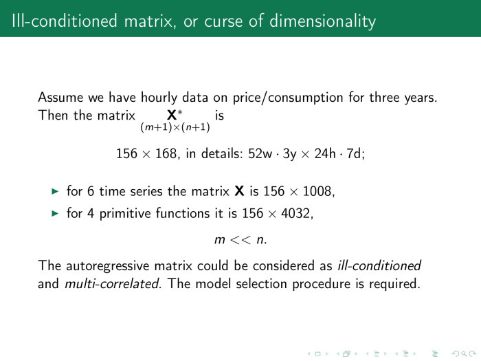
Suppose the row of matrices of the plan is a week, 7 days, 168 hours. There are data, for example, for three years. There are 52 weeks in the year. Then the three-year base matrix is 156 rows by 168 columns.
If we use six time series that I will list, that is, together with the consumption, we also take into account price, humidity, temperature, and so on, then there will be more than 1000 columns in the matrix. And if there are four more generating functions, then these are 4000 rows and 156 columns. That is, the matrix is strongly degenerate, and it is not possible to solve the linear equation normally. What to do?
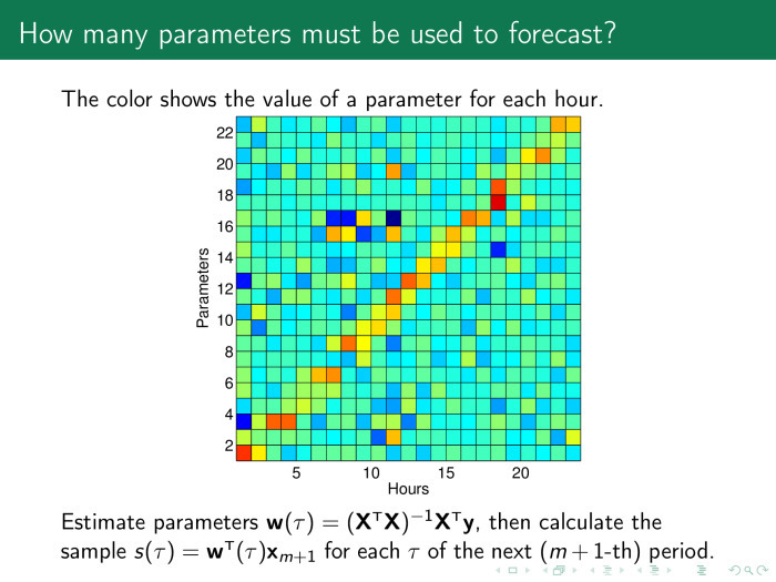
Probably, you need to run the procedure for selecting models. To do this, look at what weights make sense. For each hour we build our model, and here on the x-axis shows the values of the model parameters by the hour on the next day. And on the y-axis are the parameters themselves. We see a yellow-red diagonal, the value of the scales is larger where there is an hour in the model for the previous days.
The principle is simple. The forecast for tomorrow at 12 o'clock depends on the values for 12 hours of the previous day, the day before yesterday, and so on. Thus, we can leave only these values and throw away everything else.
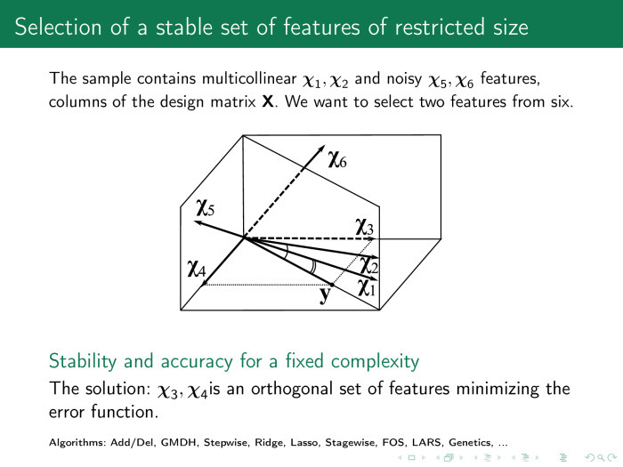
What exactly should be discarded? Imagine the matrix x as a set of columns. We approximate the time series y with a linear — or optionally linear — combination of columns of the matrix x. We would like to find a column χ that would be closer to y. A significant part of the feature selection algorithms will select the columns χ 1 and χ 2 if we want to leave two columns. But among those that we have created, we need χ 3 and χ 4 . They provide both an accurate and stable model. Exact - because the linear combination of χ 3 and χ 4 exactly approximates y, and stable - because they are orthogonal.
Why two columns? We need to see in which space we are working, how many objects are in the drawn sample. Here are three objects. Matrix x contains 3 rows and 6 columns.
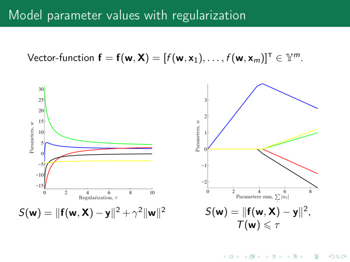
How do feature selection algorithms work? As a rule, they use error functions. In linear regression, this is the sum of the squares of the regression residuals. And there are two types of feature selection algorithms. The first type is regularizing algorithms. In addition to error, they use, as was said by Konstantin Vyacheslavovich in the last lecture, also some regularizer, a penalty on the value of the parameters and some coefficient, which is responsible for the importance of the penalty.
This coefficient can be represented in the form of such or such a fine. The weights must be no more than some value of τ.
In the first case, it is not about the loss of the number of columns in the matrix x, the number of features, but only about increasing stability. In the second case, we just lose a significant number of columns.
It is important to understand how the columns correlate with each other. How to find out?
Consider the parameter space of our model, the vector w, and calculate the value of the error at various points of w. The picture on the right shows the space itself, w 1 or w 2 . Two weights are sampled, 100 points each. It turns out 100 pairs of scales. Each point of this figure is the value of the error function. On the left, for convenience, the same is the exponent of the minus value of the error function.
It is clear that the optimal values lie somewhere in the point of 0.2–0.25 and this is what we are looking for. And the importance of the parameters is defined as follows: let's take a little bit of the parameter values from the optimal value. If we change w, the error function practically does not change. Why do we need such a parameter? Probably not needed.
Here, the value of the parameters slightly rocked along the w 2 axis, the error function dropped - fine. This basis of parameter space analysis is a way to find multi-correlating features.
Where do these signs come from? Let's look at the four main ways of generating signs. The first is the signs themselves. Where are they from? We take a time series and chop it into pieces, for example, multiples of a period. Or just by chance, or with overlap. We add these chopped segments into matrix X, the plan matrix.
The second way. Same. We transform the time series using some parametric or non-parametric features.
The third method is very interesting and promising. We are bringing pieces of the time series with some models. We will call this local modeling. And we use the parameters of these models as signs for the forecast.
Fourth. Everything happens in some kind of metric space. Let's find the centroids, cluster thickening in this space, and consider the distances from each time series to the centroids of these clusters.
Bad news. In order to build a matrix of the plan, the ratios of frequencies to sampling time series, if the series are different, should be short. In this case, the matrix of the plan grows. True, you can throw out some parts of the time series, as shown here. The entire time series “day length” is not needed, only one point per day is needed, and the plan matrix will look like this: 24 points in a row is electricity consumption, and one point and one more is the length of the daylight hours.
Here is the time series. What we have already reviewed. x ln x, in pairs, is the sum, difference, product, and various other combinations.
Here are non-parametric transformations. Just the average amount, the standard deviation. Histogram of time series quantiles.
The next option. Nonparametric transformation, Haar transform. We take the arithmetic average and put it as a single point instead of two. Or take the difference. Thus, we generate the feature and reduce the number of points in the time series, respectively, reduce the dimension of space.
The next set of generating functions is parametric functions. With them, we can approximate the time series. The first is to use this approximate series instead of the initial one. The second is to use the parameters themselves, denoted as w.
Constant, parabola, hyperbola, logarithmic sigmoid, product, power functions, exponential functions.
Another very convenient class is monotone functions. Here neural network experts can see, for example, activation functions that are often used in networks. They can be used not only at the output of networks, but also at the entrance. This also greatly improves the quality of the forecast.
The next class of generating functions is parametric time series transformations. Here we are interested in the parameters of the series themselves. We take the above functions and collect their parameters in the vector b. We have two types of parameters: the first is the parameters of the approximating functions themselves, local approximation functions, and the second vector are the model parameters, those that were considered earlier, that is, the weight parameters of linear combinations of columns of the X matrix. We can adjust them simultaneously, or we can set up iteratively and use them including as columns of the design matrix. In other words, the matrix of the plan, X, changes iteratively.
Where else can we get the parameters of the models? I will consider from the end. The splines in the approximation of the time series have parameters, nodes of splines.
Fast Fourier transforms. Instead of a time series, we can use its spectrum and also insert it into the matrix of the object – feature.
An important and well-working technique is to use the parameters of the “Singular structural analysis” or “Caterpillar” method.
This method works as follows. First, we built the matrix X - let's build a new matrix in a similar way. Now the local approximation matrix will be called H, and it will be constructed as follows: the segment of the time series enters the rows of the matrix, not one after the other, but with overlap. Let here p = 1, and k = 3. The matrix by indices will look like 1,2,3; 2,3,4; 3,4,5 and so on to the end.
Adjust the last column of the previous we will be the same method of least squares, and the coefficients used as our signs. In particular, this technique works well in determining physical activity. For example, an athlete has a watch on his arm and an athlete wants to understand how efficiently he is moving. This task is especially popular with swimmers. It is required to determine not only the type of swim, but also the power of the stroke.
The processor is weak there, no memory. And instead of solving a large problem of determining the class of a time series or predicting a series, we immediately approximate it in a similar way when we receive data. We use not an approximated time series, but approximation parameters.
This is why it works.
It shows not the time series itself, but its logged values. This point is the value of the series at a given time and one count later. It is clear that the sine will look like an ellipse. The good news is that the dimension of this ellipse in the space of logged variables will always be 2. Whatever length of prehistory we take in this space, the dimension of the space will still remain fixed. And the dimension of space can always be determined by singular decomposition.
Then we can represent each time series in the form of its main components in a singular decomposition. Accordingly, the first main component will be some kind of trend, the second - the main harmonic and so on in ascending harmonics. We use the weights of these components as attributes in approximating models.
Here is the last way to generate traits. Signs are metric. We have already somehow generated the plan matrix - let's see how its columns are located in some kind of metric space, for example, in Euclidean space.
We assign the metric ρ and cluster the rows of the object – feature matrix, X.
Naturally, the number of distances from all objects in the sample to all objects in the sample is the power of the sample in the square. Therefore, we select the centers of the clusters, measure the distance from each row to the center, and use the obtained distances as signs in the matrix of the object-attribute.
In practice, it looks like this. In order for the distance to be calculated correctly, we first align the time series. It shows six classes of rows for the accelerometer: a person goes, goes up the steps, down the steps, stands and lies. It is proposed to first align the rows with a procedure and get, for example, such rows. Next - calculate the average values or centroids for each row.
And then calculate the distance from each time series in the matrix X, the object – feature, to these centroids.
What happened as a result of generating signs in different ways? Let's look at the same data as in the beginning.
This is the data of power consumption in Poland, they are hourly. In addition, they are accompanied by different time series that describe them. We also insert gaps into this sample. Throw away some data, for example 3, 5, 10%. Fill them, and then try to predict the value of all the series at once.
On the right, we get the following object – feature matrix. On the left, time series, chopped into pieces. The first 24 time series - day. Instead of a zigzag, you should build a histogram.
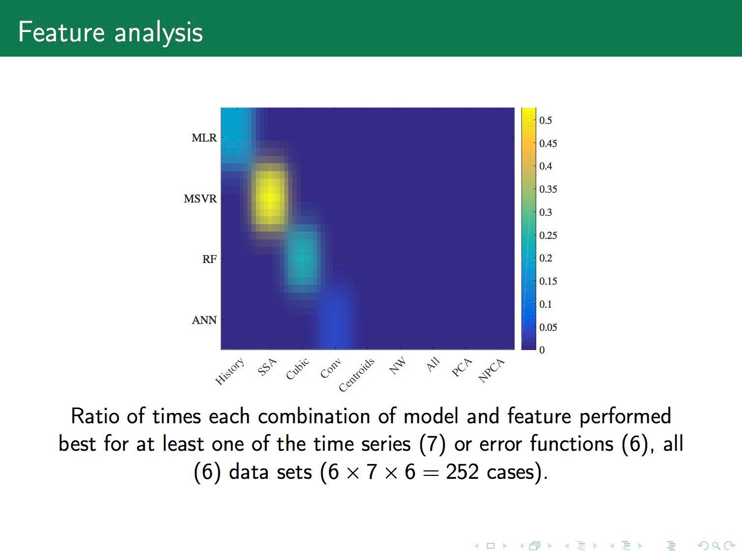
What models do we have? The best model is the forecast for tomorrow, the same as today. We will call this the base method.
Linear regression, which we considered at the beginning. Support vector machine. Neural network random forest. Of course, the fourth magic method was not enough. There are four methods that always work well, if the problem is solved at all: neural networks, support vectors, random forest and gradient boosting.
Let's compare how four different methods work with different ways of generating signs. Here again, these four ways. Historical time series. The approximation of time series. — .
. — , . — .
. . , . – , . , — . Support vector machine . random forest . .
. , support vector regression . , . , , , , . — support vector regression . , .
? , , - , . : , , - , , . , .
Source: https://habr.com/ru/post/316232/
All Articles