Will robots stand in traffic jams?

This story began with the fact that I was stuck in traffic on the highway, not particularly large, but for half an hour I stood almost in place. And, as it often happens, the traffic jam resolved on its own - there was no accident or repair ahead, just the cars at some moment began to move faster, even faster, and that’s the free road ahead.

What usually do in traffic? Well, who, when and how, and that day I was in a peaceful philosophical mood - just sat and pondered. I recalled, in particular, the post on Hiktayms about robo-mobiles, where in the comments they roughly compared the driving style of people and robots and in the end it seemed to come to the conclusion that the future is on the roads for AI, with it the traffic will become safer and the average speed will increase. Interestingly, and then there will be traffic jams? In other words, to what extent are traffic jams caused by external (objective) circumstances, and to what extent is the effect of the crowd aggressive or, on the contrary, a brake driving style? At the same time I remembered a book I had read where it was claimed that the simulation of road traffic is one of the most difficult mathematical problems, which has not yet been solved. Well, it's probably not true for a long time already, I read it a long time ago and the book was already not new at that time, it’s probably already the correct theories that were written, and everyone considered it on their computers. Although ... are there any traffic jams? In general, the flight of fancy was already unstoppable.

So, under the cut, we will try to build a more or less meaningful model of traffic on the road and, if we are lucky, we will try to simulate the difference in driving a human driver and AI. Of course, I am aware that this problem is professionally handled by entire organizations and generally very smart people, but the more interesting. And in general, set yourself unrealistic goals.

And one more thing - I am a staunch supporter of thinking with my head, therefore there will be no computer modeling in this post, in general there will be no at all, only a hardcore pencil and paper.

First we must say that there are two approaches - a microscopic model and a statistical one. The first considers the movement of each machine in a stream as a separate set of independent variables in one huge system of equations and, for obvious reasons, is most popular with theorists. The second considers the entire set as a continuous environment where each individual machine is described only as probabilistic. From a sense of contradiction from this second case, let us begin.

The simplest statistical model

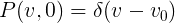
Suppose there is one strip with uniformly distributed machines with linear density ρ. However, the speeds of all machines are different, we will assume that the probability of having a speed v is described by a probability density P (v, t) depending naturally on time and equal at time t = 0 to some known function P (v, 0) . Without loss of generality, we can assume that the probability P (v, t) is defined on the interval from zero to (yes, the traffic police of all countries will forgive me) of infinity. The concepts of normalization and average ( group ) speed are also defined:

(1.1)

During the time dt, each one having speed v passes the distance vdt and can both "disappear" by catching up slower and losing speed, and "increase mass" by being caught up more quickly. It is easy to figure out that in the time interval dt, the probability of a car with speed v catching up a slower car with speed u (and slowing down) will be P (u, t) (vu) dtdu and a symmetrical expression for the probability of being caught up by a faster machine (and slowing it down). Thus, the change in probability density with time:

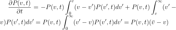(1.2)

After a little thought it is easy enough to understand that the solution should be of the form A (v) B (t) exp (-ρvt) and hence the complete solution:

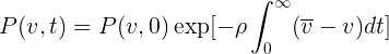(1.3)

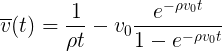
The equation turned out to be elegant, but not closed, since the average speed itself depends on time. However, we are not interested in the details of the change in the probability density P (v, t) with time, especially since they depend on an arbitrary initial function P (v, 0), so we can use (1.1) to close the equation for ̅v

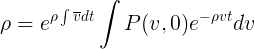and from here (1.4)
it’s already possible to work with this equation, let's consider a couple of special cases for illustration.

Let initially all cars move strictly with one speed:

from here
as it should be.

Now suppose that the velocity is distributed uniformly in a certain interval:

At the same time, the average speed drops as 1 / ta. The average distance covered increases logarithmically:

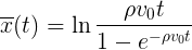- and this is good news for those who read this post while standing in traffic - you still get to the place, though in exponential time.

There is, however, one apparent contradiction - if there are cars with an arbitrarily low speed in the flow, how can the average distance traveled increase with time? The answer is that the number of cars with strictly zero speed is also zero. If we take the initial distribution in the form:

That is, almost all cars move at the same speed, and some very small part just stands, then the group velocity will fall exponentially

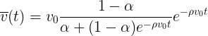
And the average distance traveled tends to a fixed limit.

Thus, we spent a couple of sheets of paper and showed that on a single-lane road, sooner or later, we would all bump into the tail of the slowest car and drag along with its speed - a brilliant result. Now let's try a slightly more realistic option.

Step towards reality

If you read carefully, to this place you should have a feeling of legitimate bewilderment - but where are the traffic jams? Why do we assume the linear density ρ to be a constant independent of neither time nor coordinate? In the end, traffic jam is essentially a cluster of cars. That's right, in our current model, we consider the motion profile averaged over a very large interval, so large that the density averaged over it is constant. Inside it, cars are knocked into columns between which there are completely empty gaps, but on the characteristic scale of our model, all this is irrelevant. The characteristic size of the heterogeneity, the column or the gap, grows with time and now, when it finally becomes equal to the characteristic scale, a traffic jam ... could arise, but does not arise, because the model is no longer applicable. We must look for a more detailed model. Please also note that for a separate machine moving in a stream there is no velocity distribution P (v, t) with which we worked before, there is only the velocity v (x, t) and the local density ρ (x, t). Here we will work with her.

First of all, the continuity equation must be satisfied for the density:

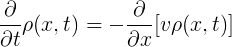(2.1)

Absolutely fundamental law essentially means that as much as a pipe has flowed in, so much should it flow out. Note that ρv is simply the number of cars crossing a section of a road per unit of time.
Of course, this equation has an infinite set of solutions, for example, it can be an arbitrary function f (x-vt) describing the motion of an arbitrary density profile with an arbitrary velocity v . If we go to the coordinate system moving along with the machine, then this expression takes an even simpler form: ρv = const . If we say the density varies according to the law ρf (x -vt) and in front of the road section with reduced speed u, u <v , then there the density profile will look like Pf (x-ut) , where ρv = Pu . Such a model is like an ideal gas and describes the ideal behavior of traffic on the road - as the speed decreases, a proportional increase in the density occurs and the number of cars crossing the cross-section of the road per unit of time is constant (up to f (x) fluctuations), you can always calculate the time for which you will pass a certain distance and it will not depend on other cars on the road.

So after all, where are the traffic jams ?

The ideal gas model describes the state of noninteracting particles; nonideality begins when interaction is taken into account. It turns out similarly with us - it is necessary to take into account the braking when the cars are too close. The braking distance can be described by the expression v ² / 2a + vτ + d , where a is the acceleration of comfortable braking estimated (roughly) by a constant; τ is the dimension of the time dimension and the order of the driver's reaction time; d - the value of the order of the length of the car.

Spatial density ρ should be the reciprocal of. It turns out? No, it is obvious that in the limit of high speeds the density should fall as 1 / v and not 1 / v ² , and we got that even the flow of cars through the cross section of the road ρv decreases with increasing speed. The mistake is that the drivers do not keep the interval inversely proportional to the stopping distance, it would be so if the car in front could stop instantly - too much assumption, in fact it brakes with the same acceleration a . Then the quadratic term disappears and a reasonable expression is obtained:

ρ _max = 1 / (vτ + d) (2.2)

as the density increases to 1 / d (that is, the bumper into the bumper), the machines can only stand, and as the speed increases, the flow tends to the limit: ρv = 1 / τ . This expression is for maximum density at a given speed , if the cars converge even more closely, they will begin to slow down. Maybe I stopped at this in too much detail, but I wanted to show how the correctly laid model begins to correct itself, reveals errors through the examination of particular and marginal cases.

Let a column of cars move along the road with the same speed v and density ρ . If this column enters the section with a reduced speed u <v , then the density of the machines increases, as we have seen before, ρ ^* = ρv / u .

However, if the density approaches critical, it may turn out that the new section of the road is unable to pass such a flow (the maximum flow of cars through the cross section of the road is ν _max (u) = uρ _max (u) = u / (uτ + d) and decreases monotonically with decreasing speed )

ρ ^* = ρv / u> ρ _max = 1 / (uτ + d) .

Now equation (2.1), which describes the change in the velocity and density profile, which however has an infinite number of solutions, including non-stationary and vibrational, comes into play. Let's take an ideal case for evaluating from above, which optimizes the road’s carrying capacity. To do this, the omniscient demon Maxwell must drive each machine, but nonetheless. Then each machine will slow down in advance at exactly the right moment to mystically guessed speed u , like this:

Moreover, the deceleration limit will move to the left with an easily calculated speed:

[ρv-u / (uτ + d)] / [1 / (uτ + d) -ρ] = [ν-ν _max (u)] / [ρ _max (u) -ρ] (2.3)

And what happens at the front? Suppose that the speed limit has disappeared at some point, then the front will begin to evaporate - the machines will begin to accelerate to the initial speed v and the front will also start moving to the left. However, the rate of evaporation is obviously less than the rate of inhibition; mainly because the driver slows down as soon as he sees the brake lights in front of him, and for acceleration he needs to estimate the distance to the car in front and its speed. It is rather difficult to estimate the rate of evaporation of a front without invoking empirical considerations; however, we can assume that it can be both more and less than the speed of the left boundary (2.3), which in turn depends on the speed limit u . And, if it turns out to be less, then we get something like a soliton on the road - a stable formation that occurs when one of the cars accidentally briefly brakes and the existing finite time. It is important to add that for the emergence of such a soliton there is no longer necessarily a real speed limit, it suffices if one of the machines spontaneously slows down for a time longer than τ to a speed less than some critical one.

There was only one small step before the traffic jams, it suffices to note that the soliton formed is unstable , its density is equal to critical (2.2) and any random sufficiently strong braking of one of the machines in the column will cause a new similar process and the formation of a new compaction with even slower speed. With a sufficiently long lifetime of such formation, this scenario will be repeated and avalanchely overlap one another until a rarefied section is reached on the road or a full stop of cars at the end of the column, which we actually observe in real life.

Now it would be possible to attract the probability theory and estimate the length of the resulting soliton (which is determined by fluctuations of the traffic density), as well as its lifetime and the likelihood of even larger seals and chances of a full stop, as well as the average decrease in road capacity. In short, based on this simple model, it is possible to construct a complete probabilistic description of road traffic. However, I suspect that I have long ago exhausted the limit on the number of formulas in a post, moreover, it would take some empirical and / or quantitative data, which I tried to avoid with all my might. Personally, I have already reached an understanding of how traffic jams happen and got some pleasure from it. In addition, I realized what an evil force had ripped out of my life for half an hour, and I immediately became better and happier to live.

What about robots?

And everything is simple with them, since I did not make any human-specific assumptions, the basic model is also true for them. That is, if robomobils are forced to go along the road at the limit of its carrying capacity, spontaneous disturbances may occur in the flow of traffic leading to deceleration up to a full stop. However, the probability of such disturbances can be tried to significantly reduce.

• First, spontaneous fluctuations occur much less frequently in a stream consisting exclusively of robots, robots do not sneeze behind the wheel, do not drop a lit cigarette, do not get distracted by the chatter of passengers and have virtually no subjective reasons to slow down. However, the objective reasons (for example, a slippery section of the road) still remain.
• Secondly, theoretically, the reaction time τ of the robot is much less, in the limit it tends to zero. However, I am afraid that the developers of robomobiles are being reinsured artificially overestimated in driving algorithms. Over time, this reserve will also be involved.
• Thirdly, emotions, in particular impatience, envy and greed are alien to robots. This allows them to keep the distance a little more than the minimum necessary, as a result, throughput decreases linearly slightly, but the probability of traffic jams nonlinearly decreases many times. However, this requires that on the road robomobili at least prevail.
• Fourth, and this is the most significant thing that distinguishes them from humans - robots are much closer to Maxwell's demons. In particular, if you allow them to share information on the road, you can create a virtual distributed AI traffic control at each site. As a simple example, a convoy of trucks can obviously win if everyone knows the speed of the first wagon in the convoy at each moment. Another one - if it becomes known that somewhere ahead (maybe far enough) compaction begins, the machines can increase the interval in advance and thus block the spread of the cork. And finally, the acceleration time can be drastically reduced if the machine receives an acceleration signal from the one ahead, which would dramatically reduce the soliton lifetime and prevent the avalanche effect.
• Finally, for those who design and build roads - do not forget that every road with a speed limit v _max has a maximum throughput capacity of the order of v _max / (τv _max + d) and if an increase in flow is expected (the city grows) at some plot to this value, it would be good to foresee the expansion of the road or an increase in maximum speed. Well, this is from the field of absolute fantasies of course.

I do not know which models are being developed by manufacturers of robots now, and in general whether they are preparing morally for the time when they will prevail on the roads; but it seems to me that it is time. It’s time to add and expand local driving algorithms to cooperative ones, and then we’ll spend less time standing in traffic jams, which means the world will be a little bit better.

PS: Initially, I planned this post on Giktimes, but was surprised to find the lack of suitable hubs. In my opinion, the right combination would be Mathematics + Interesting tasks + Transport of the future , but it turned out that the first two are present only on Habré, and in the Development section. Well, okay, I write where the hubs correspond.