Ambient Occlusion Volumes for burnt samovars
Wandering around the Internet in search of a lighting algorithm that would satisfy my needs, I came across a very new algorithm developed by NVIDIA, whose name is AOV ( Ambient Occlusion Volumes ). Having at my disposal dark autumn nights and several cups of hot coffee, I decided to study this algorithm, which resulted in this article. Before I begin, I would like to note my surprise at the fact that this algorithm has an undeservedly low popularity in the game development community, in contrast to the familiar SSAO. The content of this article will, for the most part, consist of theory.
In June 2010, Morgan McGuire , a researcher and developer at NVIDIA, developed a lighting algorithm called Ambient Occlusion Volumes . In developing this algorithm, M. McGuire, set himself the goal of achieving higher performance and quality lighting. The performance of the algorithm, according to the developer, is largely independent of the complexity of the models, and the quality of the lighting is not inferior to Ray Tracing.
AO ( Ambient Occlusion ) is an approximate to GI ( Global Illumination ) algorithm, designed to shade spaces on which, in fact, rays of light do not fall due to the fact that these spaces are conditionally overlapped by other objects, making it inaccessible for rays of light to fall into this space. The algorithm itself works by calculating the rays emanating from the point, the shading of which we check, followed by checking for the intersection of the object by the ray. If the beam passes without obstacles, then this point is illuminated, otherwise - is shaded.

But when calculating this algorithm, there are some difficulties. After some time, SSAO ( Screen Space Ambient Occlusion ) from Crytek developers came to replace the old algorithm. The algorithm itself worked according to the principle that a certain sphere is determined and in the range of this sphere, points are randomly selected and then the depths (first recorded in the depth buffer) of these points are checked from that for which we calculate the shading. If the depth of the latter is greater than the depth of a random point, then it is shaded, otherwise it is lit accordingly. Several such checks are performed, after which their results are summarized and the shading coefficient is calculated. It looks like this:
')

Due to its simplicity and, comparatively, a small load, this algorithm has become a favorite among many game developers. However, he has a lot of flaws. The main problem of this algorithm is that when checking the depth, the selected point may be outside the object that overlaps the point being checked. This leads to the fact that the point will be considered illuminated.
Further, I would like to consider another important topic before the AOV method will be described.
Many of those familiar with the name method would frown upon hearing this method in the context of Ambient Occlsuion. In fact, these methods are closely related to each other.
If you are confident in your knowledge, you have the opportunity to skip this section and proceed to the next. In the meantime, I would like to briefly go through this topic.
The radiosity method , also known as the radiance method , is one of the GI methods that relies on form-factor calculation, which, in turn, describe the exchange of energy between pairs of planes in the environment.
In short, form factors are some of the energy that is emitted from one plane and taken in by another. When calculating the form factor, the distance between the centers of the planes and the angle of rotation relative to each other is taken into account.

Calculate the form factor in this way:

where θi, j is the angle between the normal of the plane and Ri, j ,, dA1,2 is the differential region of the plane, Ri, j is the distance vector between dA1,2. In this equation, the HID is one if dA1.2 are visible to each other and zero if vice versa.
At the height of this method, two approaches were used: Full Matrix Radiosity and Progressive Refinement Radiosity .
The essence of this approach is that the environment is discretized in small planes. For each pair of planes, form factors are calculated. After that, form factors are used to create a system of equations that establishes a connection between the planes in the environment. Having solved this system, we get the intensity of the light that the plane emits. Once having calculated the intensity, the environment can be represented in any position without additional lighting calculations.
The intensity of the light that radiates a plane is calculated in this way:
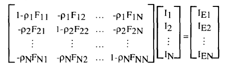
where pi is the reflection coefficient of the plane i; Fij is the form factor from the i plane to the j plane; Ii is the raidosity of the plane i; Iei is the radiation intensity of the plane i; N - the number of planes that are surrounded.
This approach was not bad, but did not allow to achieve a detailed and accurate image. In addition, it became very expensive when a large number of planes were present on the scene.
Later, this method was improved by splitting the planes into patches (fragments), and in turn each patch was broken into elements. Thus, we received a more detailed image.
The form factor from patch to patch is calculated as follows:
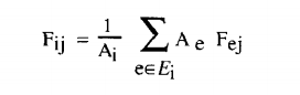
where Ei is the number of elements in the patch, Fej is the form factor from element e to patch j, Ai, e are areas of the patch and element.
This approach is based on the previous one. The peculiarity of this approach is that after each iteration there is a recalculation, namely an increment of the radiance value of the plane. It is calculated as follows:

where Ii is the already calculated radiance value.
The problem of these approaches is the complexity of calculations, even with simple forms of objects. To calculate the form factor of the plane, we need to perform two integration, not to mention the extra calculations. Hemi-Cube Radiosity has come to solve this problem.
HC is similar to the Nussalt Analog algorithm. Its essence was that around the point on the plane is located the so-called projection hemisphere with a unit radius. Another plane is projected onto this hemisphere and placed on the base of the hemisphere. Thus, the form factor will be equal to the ratio of the region of the projected plane in the base of the hemisphere to the area of the base of the hemisphere itself. The HC algorithm in its implementation uses, as you might have guessed, a semi-cube.
The sides of a semi -cube are broken down into a set of small discretized planes ( hemi-cube pixels ), each of which has its own pre-calculated form factor. When the second plane is projected onto a semi-cube, the sum of the form factors of discrete areas on which the projected plane was will be equal to the value of the form factor from a point on the first plane to the second plane.
Unfortunately, this decision had a number of its shortcomings, which became the reason for new research in this direction. If you begin to describe the shortcomings of this method, then the article will be very long, and we do not need this.
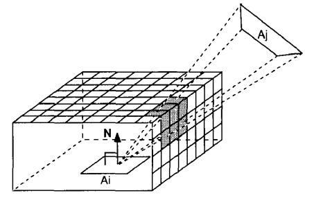
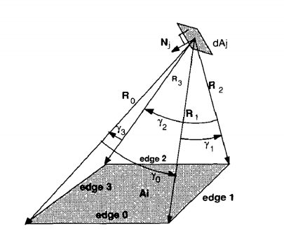
During the development of the radiosity method, Baum DR proposed this method for calculating the form factor:
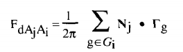
where Gi is the set of faces of the plane, Nj is the normal of the differential plane j, Gg is a value equal to the angle of gamma and the direction obtained by the vector product of Rg and R (g + 1), as shown in the figure below:
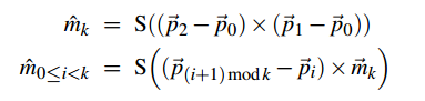
M. McGuire was inspired by this approach and based on the latter came up with an AO algorithm. He described it this way:
Let X be a very small patch of a smooth manifold. Centroid X will be at the point that is the beginning of the normal n. The polygon P will be a polygon with vertices {p0, ..., pk − 1}, which is completely located on the positive part of the plane, provided p * n> 0. Thus, the blocking of light rays created by the polygon P will be equal to the form factor emissivity between P and X.

where j = (i + 1) mod k.
In this section, I will try to consider the implementation of this algorithm from the point of view of theory. To work with this algorithm, we still need the depth and normal buffer. The following operations will occur in a geometric shader.
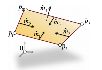
Consider a convex polygon P with vertices {p0, ..., pk − 1}, which for any combination of 3 vertices does not create collinearity. First, we need to calculate the damping function that we need to achieve smoothness when moving from near-to far-field lighting. It is calculated in this way:

where a - 1 for solid planes, m (i <k) are the normals to the faces of the polygon P, mk is the negative normal to the polygon P:
It looks like this:
The next item in our implementation will be the construction of the volume around our landfill.
To do this, we need to calculate the displacement vector, which is needed to offset the vertices of our volume relative to the vertices of the polygon.
I would like to add another new term called obscurance . It is responsible for the attenuation of the effect of overlap with the change of distance.
We obtain the displacement vector in the following way:
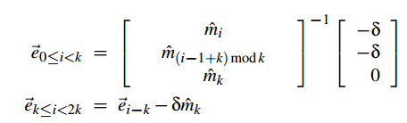
where δ is the obescurance at the maximum distance.
For clarity:
And our last step will be the product of the damping function (g) and the overlap of the polygon P (AOp (n)). Also, after all operations should be applied so-called. blending.
After all written here it would be a sin not to attach screenshots that demonstrate the work of the AOV algorithm. These screenshots were made by NVIDIA, and the demo can be found at the bottom of the article (again from NVIDIA).


For comparison with Ray Tracing:

We looked at the rather difficult way AO. Many may remain unhappy, because, most likely, they were eager to see the implementation in the form of code. Unfortunately, too much information would come out for just one article. However, those who are eager to implement this method can dig deeper from NVIDIA, which I will attach below.
PS I have a strong request to you, dear readers. If you find that the method I described in some places is incorrect or there are simply errors in terms of language, let me know, I will try to correct all my shortcomings. If you have a need to see this algorithm in the form of a code, I will try to allocate time and make a demo.
→ Demo from NVIDIA
I read a sufficient number of sources, but I focused on these particular folders:
- M. McGuire "Ambient Occlusion Volumes"
- “Improving radiosity solutions through formulated factors”
I also want to note that most of the images were taken from the last folder.
Introduction
In June 2010, Morgan McGuire , a researcher and developer at NVIDIA, developed a lighting algorithm called Ambient Occlusion Volumes . In developing this algorithm, M. McGuire, set himself the goal of achieving higher performance and quality lighting. The performance of the algorithm, according to the developer, is largely independent of the complexity of the models, and the quality of the lighting is not inferior to Ray Tracing.
A little bit about Ambient Occlusion
AO ( Ambient Occlusion ) is an approximate to GI ( Global Illumination ) algorithm, designed to shade spaces on which, in fact, rays of light do not fall due to the fact that these spaces are conditionally overlapped by other objects, making it inaccessible for rays of light to fall into this space. The algorithm itself works by calculating the rays emanating from the point, the shading of which we check, followed by checking for the intersection of the object by the ray. If the beam passes without obstacles, then this point is illuminated, otherwise - is shaded.
But when calculating this algorithm, there are some difficulties. After some time, SSAO ( Screen Space Ambient Occlusion ) from Crytek developers came to replace the old algorithm. The algorithm itself worked according to the principle that a certain sphere is determined and in the range of this sphere, points are randomly selected and then the depths (first recorded in the depth buffer) of these points are checked from that for which we calculate the shading. If the depth of the latter is greater than the depth of a random point, then it is shaded, otherwise it is lit accordingly. Several such checks are performed, after which their results are summarized and the shading coefficient is calculated. It looks like this:
')
Due to its simplicity and, comparatively, a small load, this algorithm has become a favorite among many game developers. However, he has a lot of flaws. The main problem of this algorithm is that when checking the depth, the selected point may be outside the object that overlaps the point being checked. This leads to the fact that the point will be considered illuminated.
Further, I would like to consider another important topic before the AOV method will be described.
Radiosity
Many of those familiar with the name method would frown upon hearing this method in the context of Ambient Occlsuion. In fact, these methods are closely related to each other.
If you are confident in your knowledge, you have the opportunity to skip this section and proceed to the next. In the meantime, I would like to briefly go through this topic.
The radiosity method , also known as the radiance method , is one of the GI methods that relies on form-factor calculation, which, in turn, describe the exchange of energy between pairs of planes in the environment.
In short, form factors are some of the energy that is emitted from one plane and taken in by another. When calculating the form factor, the distance between the centers of the planes and the angle of rotation relative to each other is taken into account.
Calculate the form factor in this way:
where θi, j is the angle between the normal of the plane and Ri, j ,, dA1,2 is the differential region of the plane, Ri, j is the distance vector between dA1,2. In this equation, the HID is one if dA1.2 are visible to each other and zero if vice versa.
At the height of this method, two approaches were used: Full Matrix Radiosity and Progressive Refinement Radiosity .
Full Matrix Radiosity
The essence of this approach is that the environment is discretized in small planes. For each pair of planes, form factors are calculated. After that, form factors are used to create a system of equations that establishes a connection between the planes in the environment. Having solved this system, we get the intensity of the light that the plane emits. Once having calculated the intensity, the environment can be represented in any position without additional lighting calculations.
The intensity of the light that radiates a plane is calculated in this way:
where pi is the reflection coefficient of the plane i; Fij is the form factor from the i plane to the j plane; Ii is the raidosity of the plane i; Iei is the radiation intensity of the plane i; N - the number of planes that are surrounded.
This approach was not bad, but did not allow to achieve a detailed and accurate image. In addition, it became very expensive when a large number of planes were present on the scene.
Later, this method was improved by splitting the planes into patches (fragments), and in turn each patch was broken into elements. Thus, we received a more detailed image.
The form factor from patch to patch is calculated as follows:
where Ei is the number of elements in the patch, Fej is the form factor from element e to patch j, Ai, e are areas of the patch and element.
Progressive Refinement Radiosity
This approach is based on the previous one. The peculiarity of this approach is that after each iteration there is a recalculation, namely an increment of the radiance value of the plane. It is calculated as follows:
where Ii is the already calculated radiance value.
The problem of these approaches is the complexity of calculations, even with simple forms of objects. To calculate the form factor of the plane, we need to perform two integration, not to mention the extra calculations. Hemi-Cube Radiosity has come to solve this problem.
Hemi-cube radiosity
HC is similar to the Nussalt Analog algorithm. Its essence was that around the point on the plane is located the so-called projection hemisphere with a unit radius. Another plane is projected onto this hemisphere and placed on the base of the hemisphere. Thus, the form factor will be equal to the ratio of the region of the projected plane in the base of the hemisphere to the area of the base of the hemisphere itself. The HC algorithm in its implementation uses, as you might have guessed, a semi-cube.
The sides of a semi -cube are broken down into a set of small discretized planes ( hemi-cube pixels ), each of which has its own pre-calculated form factor. When the second plane is projected onto a semi-cube, the sum of the form factors of discrete areas on which the projected plane was will be equal to the value of the form factor from a point on the first plane to the second plane.
Unfortunately, this decision had a number of its shortcomings, which became the reason for new research in this direction. If you begin to describe the shortcomings of this method, then the article will be very long, and we do not need this.
Ambient Occlusion Volume
During the development of the radiosity method, Baum DR proposed this method for calculating the form factor:
where Gi is the set of faces of the plane, Nj is the normal of the differential plane j, Gg is a value equal to the angle of gamma and the direction obtained by the vector product of Rg and R (g + 1), as shown in the figure below:
M. McGuire was inspired by this approach and based on the latter came up with an AO algorithm. He described it this way:
Let X be a very small patch of a smooth manifold. Centroid X will be at the point that is the beginning of the normal n. The polygon P will be a polygon with vertices {p0, ..., pk − 1}, which is completely located on the positive part of the plane, provided p * n> 0. Thus, the blocking of light rays created by the polygon P will be equal to the form factor emissivity between P and X.
where j = (i + 1) mod k.
AOV's implementation
In this section, I will try to consider the implementation of this algorithm from the point of view of theory. To work with this algorithm, we still need the depth and normal buffer. The following operations will occur in a geometric shader.
Consider a convex polygon P with vertices {p0, ..., pk − 1}, which for any combination of 3 vertices does not create collinearity. First, we need to calculate the damping function that we need to achieve smoothness when moving from near-to far-field lighting. It is calculated in this way:
where a - 1 for solid planes, m (i <k) are the normals to the faces of the polygon P, mk is the negative normal to the polygon P:
It looks like this:
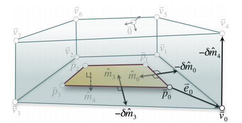
The next item in our implementation will be the construction of the volume around our landfill.
To do this, we need to calculate the displacement vector, which is needed to offset the vertices of our volume relative to the vertices of the polygon.
I would like to add another new term called obscurance . It is responsible for the attenuation of the effect of overlap with the change of distance.
We obtain the displacement vector in the following way:
where δ is the obescurance at the maximum distance.
For clarity:
And our last step will be the product of the damping function (g) and the overlap of the polygon P (AOp (n)). Also, after all operations should be applied so-called. blending.
After all written here it would be a sin not to attach screenshots that demonstrate the work of the AOV algorithm. These screenshots were made by NVIDIA, and the demo can be found at the bottom of the article (again from NVIDIA).
For comparison with Ray Tracing:
Conclusion
We looked at the rather difficult way AO. Many may remain unhappy, because, most likely, they were eager to see the implementation in the form of code. Unfortunately, too much information would come out for just one article. However, those who are eager to implement this method can dig deeper from NVIDIA, which I will attach below.
PS I have a strong request to you, dear readers. If you find that the method I described in some places is incorrect or there are simply errors in terms of language, let me know, I will try to correct all my shortcomings. If you have a need to see this algorithm in the form of a code, I will try to allocate time and make a demo.
→ Demo from NVIDIA
Literature
I read a sufficient number of sources, but I focused on these particular folders:
- M. McGuire "Ambient Occlusion Volumes"
- “Improving radiosity solutions through formulated factors”
I also want to note that most of the images were taken from the last folder.
Source: https://habr.com/ru/post/316144/
All Articles