Under exclusive conditions, we present you the full version of an article from the Hacker magazine devoted to the development on R. Under the cat you will learn how to squeeze the maximum speed when working with tabular data in R.

Note: the author’s spelling and punctuation is preserved.

What extra words? You read the article about speed, so let's get to the point right away! If you are working with a large amount of data in the project and more time is spent on transforming the tables than you would like, data.table will help solve this problem. The article will be interesting to those who are already a little familiar with the R language, as well as to developers who actively use it, but have not yet discovered the data.table package.

Install packages

Everything you need for our today's article can be installed using the appropriate functions:

  install.packages("data.table") install.packages("dplyr") install.packages("readr") 

R attacks

In recent years, the R language is deservedly gaining popularity in machine learning environments. As a rule, to work with this subsection of artificial intelligence, it is necessary to load data from several sources, carry out transformations with them to obtain a training sample, create a model on its basis, and then use this model for predictions.

In words, everything is simple, but in real life, many attempts are needed to form a “good” and sustainable model, most of which can be absolutely dead-end. The R language helps to simplify the process of creating such a model, as it is an effective tool for analyzing tabular data. To work with them in R there is a built-in data type of data.frame and a huge number of algorithms and models that actively use it. In addition, the whole power of R is the ability to extend basic functionality with third-party packages. At the time of writing, their number in the official repository reached 8914 .

But as they say, there is no limit to perfection. A large number of packages make it easier to work with the data.frame data type data.frame . Usually their goal is to simplify the syntax for performing the most common tasks. It is impossible not to recall the dplyr package, which has already become the de facto standard for working with data.frame , since due to it readability and usability of working with tables have increased significantly.

Let's data.frame from theory to practice and create a data.frame DF with columns a , b and .

  DF <- data.frame(a=sample(1:10, 100, replace = TRUE), #    1  10 b=sample(1:5, 100, replace = TRUE), #    1  5 c=100:1) #   100  1 

If we want:

• select only columns a and ,
• filter the lines, where a = 2 and > 10,
• create a new column a , equal to the sum of a and ,
• write the result to the variable DF2 ,

The basic syntax on pure data.frame will be:

  DF2 <- DF[DF$a == 2 & DF$c > 10, c("a", "c")] #     DF2$ac <- DF2$a + DF2$c #    

With dplyr everything is much dplyr :

  library(dplyr) #   dplyr DF2 <- DF %>% select(a, c) %>% filter(a == 2, c > 10) %>% mutate(ac = a + c) 

The same steps, but with comments:

  DF2 <- #  ,     DF2 DF %>% #  DF    (%>%) select(a, c) %>% #   «a»  «»    (%>%) filter(a == 2, c > 10) %>% #      (%>%) mutate(ac = a + c) #   «ac»,   «»  «» 

There is an alternative approach to working with tables - data.table . Formally, data.table is also data.frame , and it can be used with existing functions and packages, which often do not know anything about data.table and work exclusively with data.frame . This “improved” data.frame can perform many typical tasks several times faster than its progenitor. There is a legitimate question: where is the catch? This very “ambush” in data.table is its syntax, which is very different from the original. Moreover, if dplyr makes the code easier to understand from the very first seconds of use, data.table turns the code into black magic, and only years of studying witch books A few days of practice with data.table will allow data.table to fully understand the idea of ​​a new syntax and the principle of simplifying code.

We try data.table

To work with data.table you need to connect its package.

  library(data.table) #   

In further examples, these calls will be omitted and it will be assumed that the package is already loaded.

Since data is very often loaded from CSV files, data.table can be surprising at this stage. In order to show more measurable estimates, take some fairly large CSV file. As an example, one can cite data from one of the last competitions on Kaggle . There you will find a 1.27 GB training CSV file . The file structure is very simple:

• row_id - event identifier;
• x , y - coordinates;
• accuracy - accuracy;
• time - time;
• place_id is the organization identifier.

Let's try to use the basic R - read.csv and measure the time it read.csv to download this file (for this we turn to the system.time function):

  system.time( train_DF <- read.csv("train.csv") ) 

Runtime - 461.349 seconds. Enough to go for coffee ... Even if you don’t want to use data.table in the future, still try to use the built-in CSV reading functions less often. There is a good readr library, where everything is implemented much more efficiently than in basic functions. Let's look at her work on the example and connect the package.

  library(readr) 

Next, we use the function of loading data from CSV:

  system.time( train_DF <- read_csv("train.csv") ) 

Runtime - 38.067 seconds - much faster than the previous result! Let's see what data.table is capable of:

  system.time( train_DT <- fread("train.csv") ) 

The execution time is 20.906 seconds, which is almost two times faster than in readr , and twenty times faster than in the base method.

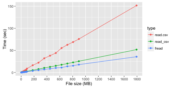
In our example, the difference in download speed for different methods was quite large. Inside each of the methods used, the time linearly depends on the file size, but the difference in speed between these methods strongly depends on the file structure (number and types of columns). Below are the test measurements of file download times.

For a file of three text columns, you can see a clear advantage of fread :

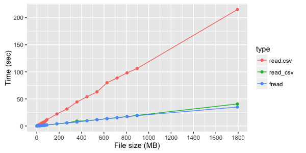
If, however, not textual, but digital columns are read, the difference between fread and read_csv less noticeable:

If after loading data from a file you are going to continue to work with data.table , then fread returns it immediately. With other ways of loading data, it will be necessary to make data.table from data.frame , although it is simple:

  train_DF #  data.frame train_DT <- data.table(train_DF) # data.table   `data.frame` 

Most speed optimizations in data.table achieved by working with objects by reference, additional copies of objects are not created in memory, which means time and resources are saved.

For example, the same task to create data.table from data.frame could be solved by one command to “pump up”, but we must remember that the initial value of the variable will be lost.

  train_DF #  data.frame setDT(train_DF) #    DF     data.table 

So, we downloaded the data, it's time to work with them. We assume that the variable DT already has a loaded data.table . The authors of the package use the following designation of the main DT[i, j, by] blocks:

• i - row filter;
• j is the choice of columns or the execution of an expression over the contents of DT ;
• by - block for grouping data.

Let us recall the very first example where we used the data.frame DF , and on it we will test various blocks. Start by creating a data.table from data.frame :

  DT <- data.table(DF) #   data.table   data.frame 

Block i - row filter

This is the most understandable of the blocks. It serves to filter the data.table rows, and if nothing else is required, you can leave out the remaining blocks.

  DT[a == 2] #    a == 2 DT[a == 2 & c > 10] #    a == 2  c > 10 

Block j - the choice of columns or the execution of an expression on the contents of data.table

This block processes the contents of data.table with filtered rows. You can simply ask to return the necessary columns by specifying them in the list . For convenience, the synonym list introduced in the form of a point (that is, list (a, b) equivalent to .(a, b) ). All existing columns in data.table are available as “variables” - you do not need to work with them as with rows, and you can use intellisense.

  DT[, list(a, c)] #   «»  «»    DT[, .(a, c)] #   

You can also specify the additional columns you want to create and assign the required values ​​to them:

  DT[, .(a, c, ac = a+c)] 

If all this is combined, you can perform the first task, which we tried to solve in different ways:

  DT2 <- DT[a == 2 & c > 10, .(a, c, ac = a + c),] 

The choice of columns is only a part of the j block capabilities. Also there you can change the existing data.table . For example, if we want to add a new column in an existing data.table , and not in a new copy (as in the previous example), this can be done using the special syntax := .

  DT2[, ac_mult2 := ac * 2] #   DT2   ac_mult2 = ac * 2 

Using the same operator, you can delete columns by assigning them to NULL .

  DT2[, ac_mult2 := NULL] #   DT2  ac_mult2 

Working with resources on the link is great, it saves power, and it is much faster, since we avoid creating a copy of the same tables with different columns. But we must understand that the change by reference changes the object itself. If you need a copy of this data in another variable, then you must explicitly indicate that it is a separate copy, and not a link to the same object.

Consider an example:

  DT3 <- DT2 DT3[, ac_mult2 := ac * 2] #    

It may seem that we have changed only DT3 , but DT2 and DT3 are one object, and, turning to DT2 , we will see a new column there. This concerns not only the deletion and creation of columns, since data.table uses references, including sorting. So the call to setorder(DT3, "a") will also affect DT2 .

To create a copy, you can use the function:

  DT3 <- copy(DT2) DT3[, ac_mult2 := NULL] 

Now DT2 and DT3 are different objects, and we deleted the column from DT3 .

by - block for grouping data

This block groups data like group_by from the dplyr or GROUP BY package in the SQL query language. The logic for accessing data.table with grouping is as follows:

1. The i block filters rows from the full data.table .
2. The by block groups the data filtered in block i by the required fields.
3. For each group, block j is executed, which can either select or update data.

The block is filled in the following way: by=list( ) , but, as in block j, list can be replaced by a point, that is, by=list(a, b) equivalent to by=.(a, b) . If you need to group only one field, you can omit the use of the list and write directly by=a :

  DT[,.(max = max(c)), by=.(a,b)] #    «a»  «b»    «max»  «» DT[,.(max = max(c)), by=a] #    «a»    «max»  «» 

The most common mistake of those who learn to work with data.table is the use of the usual data.frame constructs for data.table . This is a very sore point, and you can spend a lot of time searching for errors. If we have exactly the same data in the DF2 ( data.frame ) and DT2 ( data.table ) variables, these calls will return completely different values:

  DF2[1:5,1:2] ## ac ## 1 2 95 ## 2 2 94 ## 3 2 92 ## 4 2 80 ## 5 2 65 DT2[1:5,1:2] ## [1] 1 2 

The reason for this is very simple:

• The data.frame logic is data.frame follows - DF2[1:5,1:2] means that you need to take the first five rows and return the values ​​of the first two columns for them;
• The data.table logic data.table different - DT2[1:5,1:2] means that you need to take the first five lines and transfer them to block j. Block j will simply return 1 and 2 .

If you need to access data.table in the data.frame format, you must explicitly specify this using an additional parameter:

  DT2[1:5,1:2, with = FALSE] ## ac ## 1: 2 95 ## 2: 2 94 ## 3: 2 92 ## 4: 2 80 ## 5: 2 65 

Execution speed

Let's make sure that learning this syntax makes sense. Let's go back to the example with a large CSV file. train_DF loaded data.frame , and train_DF loaded into train_DT , respectively.

In the example used, place_id is a long integer number ( integer64 ), but only fread "guessed" this. The rest of the methods loaded this field as a floating point number, and we will need to explicitly convert the place_id field inside train_DF to compare speeds.

  install.packages("bit64") #     integer64 library(bit64) train_DF$place_id <- as.integer64(train_DF$place_id) 

Suppose we have the task of place_id number of references to each place_id in the data.

In dplyr with plain data.frame it took 13.751 seconds:

  count <- train_DF %>% #   train_DF group_by(place_id) %>% #   place_id summarise(length(place_id)) #      

At the same time, data.table does the same in 2.578 seconds:

  system.time( count2 <- train_DT[,.(.N), by = place_id] # .N -  ,      ) 

Let's complicate the task - for all place_id count the number, the median of x and y , and then sort by the number in the reverse order. data.frame c dplyr it in 27.386 seconds:

  system.time( count <- train_DF %>% #  train_DF group_by(place_id) %>% #   place_id summarise(count = length(place_id), #      mx = median(x), #   x   my = median(y)) %>% #   y   arrange(-count) #      count ) 

data.table managed much faster - 12.414 seconds:

  system.time( count2 <- train_DT[,.(count=.N, mx = median(x), my = median(y)), by = place_id][order(-count)] ) 

Test run times for simple data grouping with dplyr and data.table :

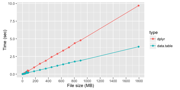
Instead of conclusions

This is only a superficial description of the data.table functionality, but it’s enough to start using this package. The dtplyr package is being dtplyr , which is positioned as a dplyr implementation for data.table , but so far it is still very young (version 0.0.1). In any case, an understanding of the features of data.table work data.table necessary before using additional “wrappers”.

about the author

Stanislav Chistyakov is an expert on cloud technologies and machine learning.

Www from author

I strongly advise reading the articles included in the package:

• Small review
• Common Questions and Answers

Www from hacker magazine

The theme of the R language is not the first time raised in our journal. Let's give you a couple of links to related articles:

• Data analysis using R. Part 1
• Studying R. Part 2: vectorization and visualization
• We program in the R language: how to write cycles for processing large amounts of data