Optimize Caffe Neural Network Platform for Intel Architecture
Modern programs that claim to be effective should take into account the specifics of the hardware on which they will be executed. In particular, we are talking about multi-core processors, for example, such as Intel Xeon and Intel Xeon Phi, large cache sizes, instruction sets, say, Intel AVX2 and Intel AVX-512, which allow for improved computing performance.

Barely resist, so as not to joke about Russiano)
For example, Caffe is a popular platform for developing deep learning neural networks. It was created at Berkley Vision and Learning Center (BVLC), it was liked by the community of independent developers who make a contribution to its development. The platform lives and develops, the proof of this is the statistics on the project page in GitHub. Caffe is called the “fast open platform for deep learning.” Is it possible to speed up such a “fast” set of tools? Asking this question, we decided to optimize Caffe for Intel architecture.
Looking ahead, thanks to integration with the Intel Math Kernel Library 2017 and a set of optimizations that we performed, following the plan outlined in this material, we started working on Intel processors more than 10 times faster than the basic version, which we, in hereinafter, we will call BVLC Caffe. The version optimized for the architecture of Intel, further, for short, will be called Intel Caffe. Here is its source code.
')
The main areas of performance improvement, details of which are described below, were to refactor code, to optimize it for using sets of vector instructions, such as Intel AVX2, to fine tune the compilation, to increase the efficiency of multi-threaded code execution using OpenMP. Tests were conducted on a system with two Intel Xeon processors. In particular, we investigated the speed of the neural network built by Caffe using the images from the CIFAR-10 set. The results of the program execution were analyzed in Intel VTune Amplifier XE 2017 and with the help of other tools.
A similar approach can be used to improve the performance of a variety of programs, for example, other platforms for deep learning of neural networks.
Before proceeding to the questions of optimization, we will discuss the algorithms of deep learning and the problems that are solved with their help.
In-depth learning algorithms are part of a more general class of machine learning algorithms, which in recent years have shown significant results in image recognition on photos and videos, in speech recognition, in natural language processing, and in other areas where you have to deal with huge amounts of information and solve data analysis problems. The success of deep learning is based on the latest advances in computing and algorithms, in the ability to handle large data sets. The principle of operation of such algorithms is that the data is passed through the layers of the network in which information is transformed, extracting more and more complex features from it.
Here is an example of how each level of the deep neural network is trained to identify the signs of increasing complexity. It shows a small set of features recognized by a deep network, rendered as images in shades of gray. It also shows the original color images, the processing of which leads to the selection of these signs. The image is taken from here .

Convolutional neural network
The work of deep learning algorithms with a teacher requires a marked set of data. Three popular types of deep neural networks that train with a teacher are multilayer perceptron (Multilayer Perceptron, MLM), convolutional neural networks (Convolution Neural Network, CNN), and recurrent neural networks (Recurrent Neural Network, RNN). In these networks, the input data, as it passes through each layer of the network, is subjected to a series of linear and non-linear transformations. As a result, the network output is generated. The network response is compared with the expected result, errors are found, then, for the output layer, the error surface gradient vector is calculated, the contribution that the synaptic weights of the neurons contribute to the network response, taking into account the activation functions, then the same procedure is performed for other layers, applying previously obtained data. This teaching method is called the backpropagation algorithm; as a result of its use, a stepwise modification of the weights of the neurons of the network is performed.
In multilayer perceptrons, the input data in each layer (represented by a vector) is first multiplied by a completely filled weighting matrix unique to the layer. In recurrent networks, such a matrix (or matrices) is the same for each layer (since the layer is recurrent), and the properties of the network depend on the input signal. Convolution networks are similar to multilayer perceptrons, but they use sparse matrices for hidden layers, called convolutional. In such networks, matrix multiplication is represented by a convolution matrix representation of the weights with a matrix representation of the input data of the layer. Convolution networks are popular in image recognition, but they are used in both speech recognition and natural language processing. Here you can read about such networks in more detail.
As already mentioned, here we are going to optimize for the Intel BVLC Caffe architecture — a popular platform for creating and researching deep learning networks. We will test the original and optimized version of the platform using the CIFAR-10 data set, which is often used in image classification problems, and the neural network model built in Caffe.

Sample images from the CIFAR-10 set
The CIFAR-10 dataset consists of 60000 color images of 32x32 pixels divided into 10 classes: plane, car, bird, cat, deer, dog, frog, horse, ship, and truck. Classes do not intersect. For example, there is no overlap between the classes "car" and "truck". “Cars” include, for example, sedans and SUVs. The “truck” class includes only heavy trucks, and, for example, pick-up trucks are not found in any group of images.
The network used during performance testing contains layers of various types. In particular, these are layers with a sigmoid activation function (such layers, in Caffe terminology, have Sigmoid type), convolutional layers (Convolution type), spatial association layers or, as they are also called, subsampling layers (Pooling type), packet normalization layers ( type BatchNorm), fully connected layers (type InnerProduct). At the output of the network is a layer with the activation function Softmax (type SoftmaxWithLoss). We will talk more about this network and its layers below. Now let's proceed to the analysis of the original version of Caffe.
One method for evaluating the performance of BVLC Caffe and Intel Caffe is to use the time command, which calculates the time it takes for the signal to travel through the layers in the forward and reverse directions. This command is very useful for measuring the time spent on calculations in each level, and to obtain a comparative execution time for different models:
In this case, “iteration” (what sets the iteration parameter) is one forward and backward pass through the batch of images. The above command displays the average execution time for 1000 iterations, both for individual layers and for the entire network. Here are the results of the work of this team for BVLC Caffe.

BVLC Caffe time command output
In the tests, we used a system with two sockets. Each had an Intel Xeon E5-2699 v3 processor (2.3 GHz) with 18 physical cores. At the same time, Intel Hyper-Threading Technology was disabled. Thus, in the system, there were only 36 physical processor cores and the same number of OpenMP threads as specified using the environment variable OMP_NUM_THREADS . Unless otherwise indicated, this configuration was used in our experiments. Please note that we recommend allowing Intel Caffe to automatically set OpenMP environment variables instead of setting them yourself. The system also has 64 GB of DDR4 memory, which operates at a frequency of 2.133 MHz.
Here are the results of performance testing, which was achieved by optimizing the code by Intel engineers. We used the following tools to measure performance:
Tools from Intel VTune Amplifier XE provide the following information:
Performance analyzes can be used to find suitable candidates for optimization, such as functions that put a heavy load on the system, and function calls that are performed for a relatively long time.
The figure below shows a summary of BVLC Caffe performance data from Intel VTune, obtained after performing 100 iterations. Elapsed Time, located at the top of the figure, is 37 seconds. This is the time it took to execute the code on the test system. CPU Time, processor time, is 1306 seconds. This is slightly less than 37 seconds, multiplied by 36 cores (1332 seconds). This indicator represents the total duration of code execution in all threads (or on all cores, since in our case Intel HT technology has been disabled), which are used in the calculations.

General results of the analysis of the performance of BVLC Caffe on the CIFAR-10 data set in the Intel VTune Amplifier XE 2017 beta
The processor utilization histogram, which is located at the bottom of the figure, indicates how often a certain number of threads are used at the same time during the test. In this case, out of 37 seconds, 14 falls on one thread (that is, on one core). All the rest of the time, we see very inefficient multi-threaded processing, with mostly less than 20 threads participating in the work.
The Top Hotspots section, located in the middle of the figure, indicates which features work the most. Here are the function calls and the contribution of each of them to the total CPU time. The kmp_fork_barrier function is an external OpenMP function, which takes 1130 seconds of CPU time to execute code. This means that about 87% of the processor's working time is spent on threads that are idle in this barrier function, without doing anything useful.
In the source code of BVLC Caffe there is a line #pragma omp parallel . However, in the code itself, there is no obvious use of the OpenMP library for organizing multi-threaded data processing. At the same time, inside Intel MKL, OpenMP streams are used to parallelize the execution of some basic mathematical calculations. In order to confirm this parallelization, we can use the Bottom-up tab in Intel VTune XE, the contents of which, after testing BVLC Caffe on the CIFAR-10 data set, are shown in the figure below. Here you can find a list of function calls and additional information about them. In particular, we are interested in the indicators of Effective Time by Utilization (the upper part of the tab) and the indicators of the distribution of the load created by the functions over the flows (the lower part).

Visualization of the time parameters of the execution of functions and the list of functions that most heavily load the system when executing BVLC Caffe on the CIFAR-10 data set
The gemm_omp_driver_v2 function is part of the libmkl_intel_thread.so library - a generic implementation of matrix multiplication (GEMM) from Intel MKL. The internal mechanisms of this function involve OpenMP multithreading. The multiplication function of matrices from Intel MKL is the main function used in the forward and backward propagation procedures, that is, in the operations of obtaining a network response and its learning. Intel MKL uses multi-threaded execution, which typically reduces GEMM computation time. However, in this particular case, the convolution operation for 32x32 images creates a not too heavy load on the system, which makes it impossible to effectively use all 36 OpenMP streams on 36 cores in one GEMM operation. Therefore, as will be shown below, the use of various multi-threading schemes and parallelization of code execution is required.
In order to demonstrate the additional load on the system, which is created by the need to work with multiple OpenMP threads, we run the same code with the environment variable OMP_NUM_THREADS = 1 , and then we compared the execution time with the previous result. What we did is shown in the figure below. Here we see the Elapsed Time indicator, equal to 31.1 seconds, instead of 37 seconds from the previous test. By writing a unit to the environment variable, we forced OpenMP to create only one thread and use it to execute the code. The resulting difference of almost six seconds indicates an additional load on the system, which is caused by the initialization and synchronization of OpenMP threads.

General results of the analysis of the performance of the BVLC Caffe on the CIFAR-10 data set in the Intel VTune Amplifier XE 2017 beta using a single stream
In the central part of the above figure there is a list of functions that most heavily load the system. Among them, we found three main candidates for optimization. Namely, these are the functions im2col_cpu , col2im_cpu , and PoolingLayer :: Forward_cpu .
Working with a CIFAR-10 dataset in a Caffe environment optimized for Intel architecture is about 13.5 times faster than using BVLC Caffe. The figure below shows the average results after 1000 iterations. On the left are BVLC Caffe data, on the right - Intel Caffe. It can be seen that in the first case, the total execution time was 270 ms, and in the second - 20 ms.

BVLC Caffe vs. Intel Caffe performance comparison
Details on how to set calculation parameters for layers can be found here .
The next section will describe the optimizations used to improve the performance of the calculations used in different layers. We followed the tutorials from the Intel Modern Code program. Some of the optimizations are based on basic math functions from Intel MKL 2017.
After profiling the BVLC Caffe code and identifying the most loaded functions that consume the most CPU time, we began work on code vectorization. Among the changes were the following:
BVLC Caffe has the ability to use Intel MKL BLAS function calls or other implementations of the same mechanisms. For example, the GEMM feature is optimized for vectorization, multi-threaded execution, and efficient use of cache memory. To improve vectorization, we also used Xbyak - JIT-assembler for x86 (IA-32) and x64 (AMD64 or x86-64) architectures. Xbyak supports the following sets of vector instructions: MMX, Intel Streaming SIMD Extensions (Intel SSE), Intel SSE2, Intel SSE3, Intel SSE4, floating point compute module, Intel AVX, Intel AVX2 and Intel AVX-512.
Xbyak is an x86 / x64 assembler for C ++, a library specially created to increase the efficiency of code execution. Xbyak is provided as a header file. It can dynamically collect mnemonic instructions for x86 and x64 architectures. JIT-generation of binary code in the process of execution provides additional optimization options. For example, this is the optimization of quantization, the operation of element-by-element division of one array into another, or the optimization of polynomial calculations due to the automatic creation of the necessary functions during program execution. With support for Intel AVX and Intel AVX2 vector instruction sets, Xbyak can achieve a better level of code vectorization in Caffe optimized for Intel architecture. The latest version of Xbyak has support for the Intel AVX-512 vector instruction set. This allows you to improve computing performance on Intel Xeon Phi x200 family processors.
Improving the performance of vectorization allows Xbyak, using SIMD instructions, to process more data at the same time, which allows for more efficient use of parallel data processing. We used Xbyak to optimize the code, which significantly improved the performance of calculations in layers of spatial union. If you know the parameters of the spatial union, you can generate assembler code for specific models of union, which uses a specific data processing window or algorithm. The result is a completely normal-looking build, which, as has been proven, works more efficiently than C ++ code compiled without using Xbyak.
Other sequential optimizations included the following:
Getting rid of repeated code execution, the results of which do not change - this is one of the scalar optimization techniques that we used. This was done in order to calculate in advance what would otherwise be calculated inside the loop with a maximum depth of nesting.
Consider, for example, this code snippet:
The third line of this fragment, for calculating the variable h_im , does not use the index of the internal cycle w_col . But despite this, the calculation of this variable is performed in each iteration of the nested loop. Alternatively, we can move this line beyond the limits of the inner loop, leading the code to this form:
Here are some additional general code optimizations that have been applied:
Intel VTune Amplifier XE found that the im2col_cpu function is one of the most heavily loaded systems. This means that she is a good candidate for performance optimization. The im2col_cpu function is the implementation of a standard step in a direct convolution operation. Each local fragment is expanded into a separate vector, the entire image is converted into a larger matrix (which increases the intensity of working with memory), the lines of which correspond to the many places where filters were applied.
One optimization technique for the im2col_cpu function is to reduce the number of operations required to access data. In the BVLC Caffe code, there are three nested loops in which the image pixels are traversed:
In this BVLC code snippet, Caffe initially calculated the corresponding indices of the array of data_col elements, although the indices of this array are simply processed sequentially. Thus, four arithmetic operations (two additions and two multiplications) can be replaced by a single index increment operation. In addition, the complexity of checking the condition can be reduced based on the following:
In the BVLC Caffe code, there was a check of a condition of the form if (x> = 0 && x <N) , where x and N are signed integers, while N is always a positive number. Converting these integers to unsigned integers allows you to change the comparison interval. Instead of performing two operations of comparing and calculating the logical AND , after the type conversion, one comparison is sufficient:
In order to avoid the operating system moving threads between compute cores, we used the OpenMP environment variable: KMP_AFFINITY = compact, granularity = fine . The compact arrangement of neighboring threads can improve the performance of GEMM operations, since threads that work together with the same last-level cache (LLC) can reuse data previously written to cache lines.
Here is the material in which you can find details about the optimization associated with blocking the cache, about the features of the optimal composition of data and vectorization.
During the use of OpenMP-parallelization, the following neural network mechanisms were optimized:
The convolution layer, which is quite consistent with its name, performs convolution of the input data using a set of weights modified during the training of the network, or filters, each of which allows to get one feature map in the output image. This optimization prevents insufficient use of hardware resources for one set of input feature maps.
We process k = min (num_threads, batch_size) of input_feature map sets . For example, k im2col operations occur in parallel and k calls are made to Intel MKL. Intel MKL switches to single-threaded execution mode automatically and overall performance is better than before when Intel MKL processed one packet. This behavior is set in the source file src / caffe / layers / base_conv_layer.cpp. This is an implementation of optimized multi-threaded processing using OpenMP from the source code file src / caffe / layers / conv_layer.cpp.
Max-pooling, average-pooling, and stochastic-pooling (not yet implemented) are different downsampling methods, while max-pooling is the most popular method. The subsample layer breaks the result obtained from the previous layer into a set of usually non-overlapping rectangular fragments. For each such fragment, the layer then outputs the maximum (max-pooling), arithmetic mean (average-pooling), or (in the future) the stochastic value (stochastic-pooling) derived from the multinomial distribution formed from the activation functions of each fragment.
The subsample layers are useful in convolutional networks for three main reasons:
, Xbyak , , . , OpenMP.
, OpenMP-. , :
collapse(2), OpenMP #pragma omp parallel for , , , .
– . , . , , , , , . softmax ( – SoftmaxWithLoss).
, , , , . , ( ), – K , j - x :
. , , . , .
, :
ReLU – , . – , (blob Caffe), , . ( – , Caffe. , Caffe ).
ReLU x x , , negative_slope :
negative_slope , ReLU, : max(x, 0) . - , :
:
S(x) = 1 / (1 + exp(-x)):
MKL ReLU-, , , ReLU- ( Xbyak). , , Intel Xeon. - . C++ .
, , , , OpenMP Intel MKL. , , , .
Caffe, Intel, CIFAR-10 Intel VTune Amplifier XE 2017 beta
Caffe, Intel, . 37 BVLC Caffe, 3.6 . 10 .
Elapsed Time, , Spin Time, , , . ( ). , , , OpenMP. OpenMP OpenMP, . , , , .
, , Caffe Intel.
Intel Modern Code
Intel VTune Amplifier XE 2017 beta , , . , , . , . , , GCC. JIT- Xbyak SIMD-.
, OpenMP, , . Intel Modern Code , , , . , , . , , -, . . Intel Xeon Phi x200 MCDRAM NUMA.
Caffe Intel , . Caffe, Intel, .
, , , , , , .
Intel OpenMP- Caffe, Intel.
Intel Modern Code .
Barely resist, so as not to joke about Russiano)
For example, Caffe is a popular platform for developing deep learning neural networks. It was created at Berkley Vision and Learning Center (BVLC), it was liked by the community of independent developers who make a contribution to its development. The platform lives and develops, the proof of this is the statistics on the project page in GitHub. Caffe is called the “fast open platform for deep learning.” Is it possible to speed up such a “fast” set of tools? Asking this question, we decided to optimize Caffe for Intel architecture.
Looking ahead, thanks to integration with the Intel Math Kernel Library 2017 and a set of optimizations that we performed, following the plan outlined in this material, we started working on Intel processors more than 10 times faster than the basic version, which we, in hereinafter, we will call BVLC Caffe. The version optimized for the architecture of Intel, further, for short, will be called Intel Caffe. Here is its source code.
')
The main areas of performance improvement, details of which are described below, were to refactor code, to optimize it for using sets of vector instructions, such as Intel AVX2, to fine tune the compilation, to increase the efficiency of multi-threaded code execution using OpenMP. Tests were conducted on a system with two Intel Xeon processors. In particular, we investigated the speed of the neural network built by Caffe using the images from the CIFAR-10 set. The results of the program execution were analyzed in Intel VTune Amplifier XE 2017 and with the help of other tools.
A similar approach can be used to improve the performance of a variety of programs, for example, other platforms for deep learning of neural networks.
Before proceeding to the questions of optimization, we will discuss the algorithms of deep learning and the problems that are solved with their help.
About deep learning algorithms
In-depth learning algorithms are part of a more general class of machine learning algorithms, which in recent years have shown significant results in image recognition on photos and videos, in speech recognition, in natural language processing, and in other areas where you have to deal with huge amounts of information and solve data analysis problems. The success of deep learning is based on the latest advances in computing and algorithms, in the ability to handle large data sets. The principle of operation of such algorithms is that the data is passed through the layers of the network in which information is transformed, extracting more and more complex features from it.
Here is an example of how each level of the deep neural network is trained to identify the signs of increasing complexity. It shows a small set of features recognized by a deep network, rendered as images in shades of gray. It also shows the original color images, the processing of which leads to the selection of these signs. The image is taken from here .
Convolutional neural network
The work of deep learning algorithms with a teacher requires a marked set of data. Three popular types of deep neural networks that train with a teacher are multilayer perceptron (Multilayer Perceptron, MLM), convolutional neural networks (Convolution Neural Network, CNN), and recurrent neural networks (Recurrent Neural Network, RNN). In these networks, the input data, as it passes through each layer of the network, is subjected to a series of linear and non-linear transformations. As a result, the network output is generated. The network response is compared with the expected result, errors are found, then, for the output layer, the error surface gradient vector is calculated, the contribution that the synaptic weights of the neurons contribute to the network response, taking into account the activation functions, then the same procedure is performed for other layers, applying previously obtained data. This teaching method is called the backpropagation algorithm; as a result of its use, a stepwise modification of the weights of the neurons of the network is performed.
In multilayer perceptrons, the input data in each layer (represented by a vector) is first multiplied by a completely filled weighting matrix unique to the layer. In recurrent networks, such a matrix (or matrices) is the same for each layer (since the layer is recurrent), and the properties of the network depend on the input signal. Convolution networks are similar to multilayer perceptrons, but they use sparse matrices for hidden layers, called convolutional. In such networks, matrix multiplication is represented by a convolution matrix representation of the weights with a matrix representation of the input data of the layer. Convolution networks are popular in image recognition, but they are used in both speech recognition and natural language processing. Here you can read about such networks in more detail.
Caffe, CIFAR-10 and image classification
As already mentioned, here we are going to optimize for the Intel BVLC Caffe architecture — a popular platform for creating and researching deep learning networks. We will test the original and optimized version of the platform using the CIFAR-10 data set, which is often used in image classification problems, and the neural network model built in Caffe.
Sample images from the CIFAR-10 set
The CIFAR-10 dataset consists of 60000 color images of 32x32 pixels divided into 10 classes: plane, car, bird, cat, deer, dog, frog, horse, ship, and truck. Classes do not intersect. For example, there is no overlap between the classes "car" and "truck". “Cars” include, for example, sedans and SUVs. The “truck” class includes only heavy trucks, and, for example, pick-up trucks are not found in any group of images.
The network used during performance testing contains layers of various types. In particular, these are layers with a sigmoid activation function (such layers, in Caffe terminology, have Sigmoid type), convolutional layers (Convolution type), spatial association layers or, as they are also called, subsampling layers (Pooling type), packet normalization layers ( type BatchNorm), fully connected layers (type InnerProduct). At the output of the network is a layer with the activation function Softmax (type SoftmaxWithLoss). We will talk more about this network and its layers below. Now let's proceed to the analysis of the original version of Caffe.
Initial performance analysis
One method for evaluating the performance of BVLC Caffe and Intel Caffe is to use the time command, which calculates the time it takes for the signal to travel through the layers in the forward and reverse directions. This command is very useful for measuring the time spent on calculations in each level, and to obtain a comparative execution time for different models:
./build/tools/caffe time \ --model=examples/cifar10/cifar10_full_sigmoid_train_test_bn.prototxt \ -iterations 1000 In this case, “iteration” (what sets the iteration parameter) is one forward and backward pass through the batch of images. The above command displays the average execution time for 1000 iterations, both for individual layers and for the entire network. Here are the results of the work of this team for BVLC Caffe.
BVLC Caffe time command output
In the tests, we used a system with two sockets. Each had an Intel Xeon E5-2699 v3 processor (2.3 GHz) with 18 physical cores. At the same time, Intel Hyper-Threading Technology was disabled. Thus, in the system, there were only 36 physical processor cores and the same number of OpenMP threads as specified using the environment variable OMP_NUM_THREADS . Unless otherwise indicated, this configuration was used in our experiments. Please note that we recommend allowing Intel Caffe to automatically set OpenMP environment variables instead of setting them yourself. The system also has 64 GB of DDR4 memory, which operates at a frequency of 2.133 MHz.
Here are the results of performance testing, which was achieved by optimizing the code by Intel engineers. We used the following tools to measure performance:
- Callgrind from the Valgrind toolkit.
- Intel VTune Amplifier XE 2017 beta.
Tools from Intel VTune Amplifier XE provide the following information:
- Functions that create the greatest load on the system (hotspots).
- System calls (including task switching).
- CPU and cache usage.
- Load distribution across OpenMP threads.
- Thread locks
- Memory usage.
Performance analyzes can be used to find suitable candidates for optimization, such as functions that put a heavy load on the system, and function calls that are performed for a relatively long time.
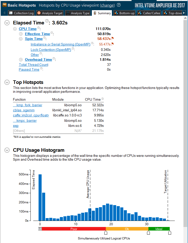
The figure below shows a summary of BVLC Caffe performance data from Intel VTune, obtained after performing 100 iterations. Elapsed Time, located at the top of the figure, is 37 seconds. This is the time it took to execute the code on the test system. CPU Time, processor time, is 1306 seconds. This is slightly less than 37 seconds, multiplied by 36 cores (1332 seconds). This indicator represents the total duration of code execution in all threads (or on all cores, since in our case Intel HT technology has been disabled), which are used in the calculations.
General results of the analysis of the performance of BVLC Caffe on the CIFAR-10 data set in the Intel VTune Amplifier XE 2017 beta
The processor utilization histogram, which is located at the bottom of the figure, indicates how often a certain number of threads are used at the same time during the test. In this case, out of 37 seconds, 14 falls on one thread (that is, on one core). All the rest of the time, we see very inefficient multi-threaded processing, with mostly less than 20 threads participating in the work.
The Top Hotspots section, located in the middle of the figure, indicates which features work the most. Here are the function calls and the contribution of each of them to the total CPU time. The kmp_fork_barrier function is an external OpenMP function, which takes 1130 seconds of CPU time to execute code. This means that about 87% of the processor's working time is spent on threads that are idle in this barrier function, without doing anything useful.
In the source code of BVLC Caffe there is a line #pragma omp parallel . However, in the code itself, there is no obvious use of the OpenMP library for organizing multi-threaded data processing. At the same time, inside Intel MKL, OpenMP streams are used to parallelize the execution of some basic mathematical calculations. In order to confirm this parallelization, we can use the Bottom-up tab in Intel VTune XE, the contents of which, after testing BVLC Caffe on the CIFAR-10 data set, are shown in the figure below. Here you can find a list of function calls and additional information about them. In particular, we are interested in the indicators of Effective Time by Utilization (the upper part of the tab) and the indicators of the distribution of the load created by the functions over the flows (the lower part).
Visualization of the time parameters of the execution of functions and the list of functions that most heavily load the system when executing BVLC Caffe on the CIFAR-10 data set
The gemm_omp_driver_v2 function is part of the libmkl_intel_thread.so library - a generic implementation of matrix multiplication (GEMM) from Intel MKL. The internal mechanisms of this function involve OpenMP multithreading. The multiplication function of matrices from Intel MKL is the main function used in the forward and backward propagation procedures, that is, in the operations of obtaining a network response and its learning. Intel MKL uses multi-threaded execution, which typically reduces GEMM computation time. However, in this particular case, the convolution operation for 32x32 images creates a not too heavy load on the system, which makes it impossible to effectively use all 36 OpenMP streams on 36 cores in one GEMM operation. Therefore, as will be shown below, the use of various multi-threading schemes and parallelization of code execution is required.
In order to demonstrate the additional load on the system, which is created by the need to work with multiple OpenMP threads, we run the same code with the environment variable OMP_NUM_THREADS = 1 , and then we compared the execution time with the previous result. What we did is shown in the figure below. Here we see the Elapsed Time indicator, equal to 31.1 seconds, instead of 37 seconds from the previous test. By writing a unit to the environment variable, we forced OpenMP to create only one thread and use it to execute the code. The resulting difference of almost six seconds indicates an additional load on the system, which is caused by the initialization and synchronization of OpenMP threads.
General results of the analysis of the performance of the BVLC Caffe on the CIFAR-10 data set in the Intel VTune Amplifier XE 2017 beta using a single stream
In the central part of the above figure there is a list of functions that most heavily load the system. Among them, we found three main candidates for optimization. Namely, these are the functions im2col_cpu , col2im_cpu , and PoolingLayer :: Forward_cpu .
Code optimization
Working with a CIFAR-10 dataset in a Caffe environment optimized for Intel architecture is about 13.5 times faster than using BVLC Caffe. The figure below shows the average results after 1000 iterations. On the left are BVLC Caffe data, on the right - Intel Caffe. It can be seen that in the first case, the total execution time was 270 ms, and in the second - 20 ms.
BVLC Caffe vs. Intel Caffe performance comparison
Details on how to set calculation parameters for layers can be found here .
The next section will describe the optimizations used to improve the performance of the calculations used in different layers. We followed the tutorials from the Intel Modern Code program. Some of the optimizations are based on basic math functions from Intel MKL 2017.
Scalar and sequential optimization
▍ Code vectorization
After profiling the BVLC Caffe code and identifying the most loaded functions that consume the most CPU time, we began work on code vectorization. Among the changes were the following:
- Improved work with libraries of Basic Linear Algebra Subprograms (BLAS), namely - the transition from Automatically Tuned Linear Algebra System (ATLAS) to Intel MKL.
- Optimization in the process of assembling code (using JIT-assembler Xbyak).
- Code vectorization using GNU Compiler Collection (GCC) and OpenMP.
BVLC Caffe has the ability to use Intel MKL BLAS function calls or other implementations of the same mechanisms. For example, the GEMM feature is optimized for vectorization, multi-threaded execution, and efficient use of cache memory. To improve vectorization, we also used Xbyak - JIT-assembler for x86 (IA-32) and x64 (AMD64 or x86-64) architectures. Xbyak supports the following sets of vector instructions: MMX, Intel Streaming SIMD Extensions (Intel SSE), Intel SSE2, Intel SSE3, Intel SSE4, floating point compute module, Intel AVX, Intel AVX2 and Intel AVX-512.
Xbyak is an x86 / x64 assembler for C ++, a library specially created to increase the efficiency of code execution. Xbyak is provided as a header file. It can dynamically collect mnemonic instructions for x86 and x64 architectures. JIT-generation of binary code in the process of execution provides additional optimization options. For example, this is the optimization of quantization, the operation of element-by-element division of one array into another, or the optimization of polynomial calculations due to the automatic creation of the necessary functions during program execution. With support for Intel AVX and Intel AVX2 vector instruction sets, Xbyak can achieve a better level of code vectorization in Caffe optimized for Intel architecture. The latest version of Xbyak has support for the Intel AVX-512 vector instruction set. This allows you to improve computing performance on Intel Xeon Phi x200 family processors.
Improving the performance of vectorization allows Xbyak, using SIMD instructions, to process more data at the same time, which allows for more efficient use of parallel data processing. We used Xbyak to optimize the code, which significantly improved the performance of calculations in layers of spatial union. If you know the parameters of the spatial union, you can generate assembler code for specific models of union, which uses a specific data processing window or algorithm. The result is a completely normal-looking build, which, as has been proven, works more efficiently than C ++ code compiled without using Xbyak.
▍General code optimization
Other sequential optimizations included the following:
- Reducing the complexity of algorithms.
- Reducing the amount of computation.
- Unrolling loops.
Getting rid of repeated code execution, the results of which do not change - this is one of the scalar optimization techniques that we used. This was done in order to calculate in advance what would otherwise be calculated inside the loop with a maximum depth of nesting.
Consider, for example, this code snippet:
for (int h_col = 0; h_col < height_col; ++h_col) { for (int w_col = 0; w_col < width_col; ++w_col) { int h_im = h_col * stride_h - pad_h + h_offset; int w_im = w_col * stride_w - pad_w + w_offset; The third line of this fragment, for calculating the variable h_im , does not use the index of the internal cycle w_col . But despite this, the calculation of this variable is performed in each iteration of the nested loop. Alternatively, we can move this line beyond the limits of the inner loop, leading the code to this form:
for (int h_col = 0; h_col < height_col; ++h_col) { int h_im = h_col * stride_h - pad_h + h_offset; for (int w_col = 0; w_col < width_col; ++w_col) { int w_im = w_col * stride_w - pad_w + w_offset; Processor-specific optimizations, systems, and other general approaches to improving code
Here are some additional general code optimizations that have been applied:
- Improved implementation of the im2col_cpu and col2im_cpu functions .
- Reducing the complexity of the batch normalization operation.
- CPU and system specific optimizations.
- Using a single core per computing thread.
- Elimination of movement of threads between computational cores.
Intel VTune Amplifier XE found that the im2col_cpu function is one of the most heavily loaded systems. This means that she is a good candidate for performance optimization. The im2col_cpu function is the implementation of a standard step in a direct convolution operation. Each local fragment is expanded into a separate vector, the entire image is converted into a larger matrix (which increases the intensity of working with memory), the lines of which correspond to the many places where filters were applied.
One optimization technique for the im2col_cpu function is to reduce the number of operations required to access data. In the BVLC Caffe code, there are three nested loops in which the image pixels are traversed:
for (int c_col = 0; c_col < channels_col; ++c_col) for (int h_col = 0; h_col < height_col; ++h_col) for (int w_col = 0; w_col < width_col; ++w_col) data_col[(c_col*height_col+h_col)*width_col+w_col] = // ... In this BVLC code snippet, Caffe initially calculated the corresponding indices of the array of data_col elements, although the indices of this array are simply processed sequentially. Thus, four arithmetic operations (two additions and two multiplications) can be replaced by a single index increment operation. In addition, the complexity of checking the condition can be reduced based on the following:
/* int unsigned , a , , b. b – unsigned, , , , 0x800…, , , 0x800… . */ inline bool is_a_ge_zero_and_a_lt_b(int a, int b) { return static_cast<unsigned>(a) < static_cast<unsigned>(b); } In the BVLC Caffe code, there was a check of a condition of the form if (x> = 0 && x <N) , where x and N are signed integers, while N is always a positive number. Converting these integers to unsigned integers allows you to change the comparison interval. Instead of performing two operations of comparing and calculating the logical AND , after the type conversion, one comparison is sufficient:
if (((unsigned) x) < ((unsigned) N)) In order to avoid the operating system moving threads between compute cores, we used the OpenMP environment variable: KMP_AFFINITY = compact, granularity = fine . The compact arrangement of neighboring threads can improve the performance of GEMM operations, since threads that work together with the same last-level cache (LLC) can reuse data previously written to cache lines.
Here is the material in which you can find details about the optimization associated with blocking the cache, about the features of the optimal composition of data and vectorization.
Code parallelization using OpenMP
▍ Neural network layers
During the use of OpenMP-parallelization, the following neural network mechanisms were optimized:
- Convolution Layer (Convolution).
- Deconvolution transformation layer.
- Local normalization layer (LRN).
- Layer with a semi-linear activation function (Rectified-Linear Unit, ReLU)
- Layer with Softmax activation function.
- Concatenation layer.
- Utilities for OpenBLAS optimization, such as the vPowx operation - y [i] = x [i] β, the operations caffe_set , caffe_copy , and caffe_rng_bernoulli .
- The layer of spatial union, or subsamples (Pooling).
- Layer “thinning” network to prevent the effect of retraining (Dropout).
- Batch normalization layer.
- Data layer.
- Layer for performing elementwise operations (Eltwise).
Configuration layer
The convolution layer, which is quite consistent with its name, performs convolution of the input data using a set of weights modified during the training of the network, or filters, each of which allows to get one feature map in the output image. This optimization prevents insufficient use of hardware resources for one set of input feature maps.
template <typename Dtype> void ConvolutionLayer<Dtype>::Forward_cpu(const vector<Blob<Dtype>*>& \ bottom, const vector<Blob<Dtype>*>& top) { const Dtype* weight = this->blobs_[0]->cpu_data(); // , , // ( , 36 // ). // MKL. for (int i = 0; i < bottom.size(); ++i) { const Dtype* bottom_data = bottom[i]->cpu_data(); Dtype* top_data = top[i]->mutable_cpu_data(); #ifdef _OPENMP #pragma omp parallel for num_threads(this->num_of_threads_) #endif for (int n = 0; n < this->num_; ++n) { this->forward_cpu_gemm(bottom_data + n*this->bottom_dim_, weight, top_data + n*this->top_dim_); if (this->bias_term_) { const Dtype* bias = this->blobs_[1]->cpu_data(); this->forward_cpu_bias(top_data + n * this->top_dim_, bias); } } } } We process k = min (num_threads, batch_size) of input_feature map sets . For example, k im2col operations occur in parallel and k calls are made to Intel MKL. Intel MKL switches to single-threaded execution mode automatically and overall performance is better than before when Intel MKL processed one packet. This behavior is set in the source file src / caffe / layers / base_conv_layer.cpp. This is an implementation of optimized multi-threaded processing using OpenMP from the source code file src / caffe / layers / conv_layer.cpp.
Subsample layer
Max-pooling, average-pooling, and stochastic-pooling (not yet implemented) are different downsampling methods, while max-pooling is the most popular method. The subsample layer breaks the result obtained from the previous layer into a set of usually non-overlapping rectangular fragments. For each such fragment, the layer then outputs the maximum (max-pooling), arithmetic mean (average-pooling), or (in the future) the stochastic value (stochastic-pooling) derived from the multinomial distribution formed from the activation functions of each fragment.
The subsample layers are useful in convolutional networks for three main reasons:
- The subsample reduces the dimension of the problem and the computational load on the overlying layers.
- The subsample for the underlying layers allows the convolution kernels in the layers above to cover large areas of input data, and thus learn more complex features. For example, the core of a layer below is usually trained to recognize small elements of the image, while the core of a layer above can be trained to recognize more complex structures, such as images of forests or beaches.
- The max-pooling method increases the stability of the network to image shift. 2x2 ( ) , . 3x3 .
, Xbyak , , . , OpenMP.
, OpenMP-. , :
#ifdef _OPENMP #pragma omp parallel for collapse(2) #endif for (int image = 0; image < num_batches; ++image) for (int channel = 0; channel < num_channels; ++channel) generator_func(bottom_data, top_data, top_count, image, image+1, mask, channel, channel+1, this, use_top_mask); } collapse(2), OpenMP #pragma omp parallel for , , , .
▍ Softmax
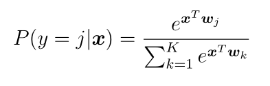
– . , . , , , , , . softmax ( – SoftmaxWithLoss).
, , , , . , ( ), – K , j - x :
. , , . , .
, :
// #ifdef _OPENMP #pragma omp parallel for #endif for (int j = 0; j < channels; j++) { caffe_div(inner_num_, top_data + j*inner_num_, scale_data, top_data + j*inner_num_); } ▍ReLU
ReLU – , . – , (blob Caffe), , . ( – , Caffe. , Caffe ).
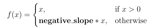
ReLU x x , , negative_slope :
negative_slope , ReLU, : max(x, 0) . - , :
template <typename Dtype> void ReLULayer<Dtype>::Forward_cpu(const vector<Blob<Dtype>*>& bottom, const vector<Blob<Dtype>*>& top) { const Dtype* bottom_data = bottom[0]->cpu_data(); Dtype* top_data = top[0]->mutable_cpu_data(); const int count = bottom[0]->count(); Dtype negative_slope=this->layer_param_.relu_param().negative_slope(); #ifdef _OPENMP #pragma omp parallel for #endif for (int i = 0; i < count; ++i) { top_data[i] = std::max(bottom_data[i], Dtype(0)) + negative_slope * std::min(bottom_data[i], Dtype(0)); } } :
template <typename Dtype> void ReLULayer<Dtype>::Backward_cpu(const vector<Blob<Dtype>*>& top, const vector<bool>& propagate_down, const vector<Blob<Dtype>*>& bottom) { if (propagate_down[0]) { const Dtype* bottom_data = bottom[0]->cpu_data(); const Dtype* top_diff = top[0]->cpu_diff(); Dtype* bottom_diff = bottom[0]->mutable_cpu_diff(); const int count = bottom[0]->count(); Dtype negative_slope=this->layer_param_.relu_param().negative_slope(); #ifdef _OPENMP #pragma omp parallel for #endif for (int i = 0; i < count; ++i) { bottom_diff[i] = top_diff[i] * ((bottom_data[i] > 0) + negative_slope * (bottom_data[i] <= 0)); } } } S(x) = 1 / (1 + exp(-x)):
#ifdef _OPENMP #pragma omp parallel for #endif for (int i = 0; i < count; ++i) { top_data[i] = sigmoid(bottom_data[i]); } MKL ReLU-, , , ReLU- ( Xbyak). , , Intel Xeon. - . C++ .
findings
, , , , OpenMP Intel MKL. , , , .
Caffe, Intel, CIFAR-10 Intel VTune Amplifier XE 2017 beta
Caffe, Intel, . 37 BVLC Caffe, 3.6 . 10 .
Elapsed Time, , Spin Time, , , . ( ). , , , OpenMP. OpenMP OpenMP, . , , , .
, , Caffe Intel.
Intel Modern Code
Intel VTune Amplifier XE 2017 beta , , . , , . , . , , GCC. JIT- Xbyak SIMD-.
, OpenMP, , . Intel Modern Code , , , . , , . , , -, . . Intel Xeon Phi x200 MCDRAM NUMA.
Caffe Intel , . Caffe, Intel, .
, , , , , , .
Intel OpenMP- Caffe, Intel.
Intel Modern Code .
Source: https://habr.com/ru/post/315582/
All Articles