Deep learning for newbies: fine tuning neural network

Introduction

Introducing the third (and latest) article in a series designed to help you quickly understand deep learning technology; we will move from basic principles to non-trivial features in order to get decent performance on two data sets: MNIST (handwritten classification) and CIFAR-10 (classification of small images into ten classes: airplane, car, bird, cat, deer, dog, frog , horse, ship and truck).


Last time, we looked at the convolutional neural network model and showed how using a simple but effective regularization method called dropout, you can quickly reach an accuracy of 78.6% using the Keras deep learning network framework.

You now have the basic skills required to apply in-depth training to most interesting tasks (an exception is the task of processing non - linear time series , which is beyond the scope of this manual, and for which recurrent neural networks (RNN) are usually preferable.) The final part of this manual will contain what is very important, but is often overlooked in such articles — tricks and tricks of fine-tuning the model to teach it to generalize better than the basic model with which you started.

This part of the manual assumes familiarity with the first and second articles of the cycle.
')

Configuring hyperparameters and base model

Typically, the process of developing a neural network begins with the development of a simple network, either directly using those architectures that have already been successfully used to solve such problems, or using those hyperparameters that have previously produced good results. Ultimately, we hope, we will reach a level of performance that will serve as a good starting point, after which we can try to change all the fixed parameters and extract the maximum performance from the network. This process is commonly referred to as setting up hyper parameters , because it involves changing the network components that must be installed before starting the training.

Although the method described here may provide more tangible benefits on the CIFAR-10, due to the relative complexity of quickly creating a prototype on it in the absence of a graphics processor, we will focus on improving its performance on MNIST. Of course, if resources allow, I encourage you to try out similar methods on CIFAR and see with your own eyes how much they gain compared to the standard CNN approach.

The starting point for us will be the original CNN, presented below. If any code fragments seem incomprehensible to you, I suggest to get acquainted with the previous two parts of this cycle, where all the basic principles are described.



As you can see, our model achieves an accuracy of 99.12% on the test set. This is slightly better than the results of the MLP, discussed in the first part, but we still have room to grow!

In this guide, we will share ways to improve such “basic” neural networks (without departing from the CNN architecture), and then we will evaluate the performance gains that we will receive.

-regularization

In the previous article, we said that one of the main problems of machine learning is the problem of overfitting , when the model in the pursuit of minimizing training costs loses the ability to generalize.


As already mentioned, there is an easy way to keep retraining under control - the dropout method.

But there are other regularizers that can be applied to our network. Perhaps the most popular of them is -regularization (also called weight reduction, weight decay), which uses a more direct approach to regularization than the dropout. Usually, the root cause of retraining is the complexity of the model (in terms of the number of its parameters), which is too high for the problem being solved and the training set available. In a sense, the task of the regularizer is to reduce the complexity of the model, while maintaining the number of its parameters. -regularization is performed by imposing fines (penalizing) on ​​the weights with the highest values, minimizing them -normal using the parameter λ - the regularization coefficient, which expresses a preference for minimizing the norm with respect to minimizing losses on the training set. That is, for each weight ω we add to the objective function addend (the factor ½ is used so that the gradient of this term in the parameter ω equals λω, and not 2λω - for the convenience of applying the backpropagation method).

Please note that it is crucial to choose the right λ. If the coefficient is too small, the effect of regularization will be negligible, but if it is too large, the model will reset all weights. Here we take λ = 0.0001; to add this regularization method to our model, we need one more import, after which it is enough just to add the W_regularizer parameter to each layer where we want to apply regularization.

 from keras.regularizers import l2 # L2-regularisation # ... l2_lambda = 0.0001 # ... # This is how to add L2-regularisation to any Keras layer with weights (eg Convolution2D/Dense) conv_1 = Convolution2D(conv_depth, kernel_size, kernel_size, border_mode='same', W_regularizer=l2(l2_lambda), activation='relu')(inp) 

Network initialization

One of the moments that we lost sight of in the previous article is the principle of choosing the initial weights for the layers that make up the model. Obviously, this question is very important: setting all weights to 0 will be a serious obstacle to learning, since none of the weights will initially be active. Assigning values ​​from the interval of ± 1 to the weights is also usually not the best option - in fact, sometimes (depending on the task and complexity of the model), the correct model initialization may depend on whether it reaches the highest performance or does not converge at all. Even if the task does not imply such an extreme, the successfully chosen method of initializing the scales can significantly affect the model's ability to learn, since it presets the model parameters taking into account the loss function.

Here I will give the two most interesting methods.

Xavier initialization method (sometimes the Glorot method). The main idea of ​​this method is to simplify the passage of the signal through the layer during both direct and reverse propagation of errors for the linear activation function (this method also works well for the sigmoid function, since the section where it is unsaturated is also linear). When calculating weights, this method relies on a probability distribution (uniform or normal) with a variance equal to where and - the number of neurons in the previous and subsequent layers, respectively.

The Ge (He) initialization method is a variation of the Zawier method, more appropriate for the ReLU activation function, compensating for the fact that this function returns zero for half of the definition domain. Namely, in this case

To obtain the desired variance for initializing Zavier, consider what happens to the variance of the output values ​​of a linear neuron (without the displacement component), assuming that the weights and input values do not correlate and have a zero expectation :

From this it follows that in order to preserve the dispersion of the input data after passing through the layer, it is necessary that the dispersion be . We can use the same argument in back propagation of an error to get . Since we usually cannot meet both of these requirements, we choose the dispersion of weights as their average: That in practice usually works great.

These two methods are suitable for most of the examples that you come across (although research also deserves the orthogonal initialization method, especially with respect to recurrent networks). It is not difficult to specify the initialization method for the layer: you just need to specify the init parameter, as described below. We will use a uniform Ge initialization ( he_uniform ) for all ReLU layers and a uniform Zawier initialization ( glorot_uniform ) for the output softmax layer (since in essence it is a generalization of the logistic function to multiple similar data).

 # Add He initialisation to a layer conv_1 = Convolution2D(conv_depth, kernel_size, kernel_size, border_mode='same', init='he_uniform', W_regularizer=l2(l2_lambda), activation='relu')(inp) # Add Xavier initialisation to a layer out = Dense(num_classes, init='glorot_uniform', W_regularizer=l2(l2_lambda), activation='softmax')(drop) 

Batch normalization (batch normalization)

Butch normalization is a method of accelerating deep learning proposed by Ioffe and Szegedy in early 2015, already quoted on arXiv 560 times! The method solves the following problem, which impedes the effective training of neural networks: as the signal propagates through the network, even if we normalize it at the input, passing through the inner layers, it can be greatly distorted both by the mean and the dispersion (this phenomenon is called the internal covariance shift ), which is fraught with serious inconsistencies between gradients at different levels. Therefore, we have to use stronger regularizers, thereby slowing down the pace of learning.

Butch normalization offers a very simple solution to this problem: to normalize the input data in such a way as to get a zero expectation and unit variance. Normalization is performed before entering each layer. This means that during training we normalize batch_size examples, and during testing we normalize the statistics obtained from the entire training set, since we cannot see the test data in advance. Namely, we calculate the expectation and variance for a specific batch (package) in the following way:

Using these statistical characteristics, we transform the activation function in such a way that it has zero expectation and unit variance over the entire batch:

where ε> 0 is the parameter that protects us from division by 0 (in case the standard deviation of the batch is very small or even zero). Finally, to get the final activation function y , we need to make sure that during normalization we did not lose the ability to generalize, and since we applied scaling and shifting operations to the original data, we can allow arbitrary scaling and shifting of normalized values, having obtained the final function activation:

Where β and γ are the parameters of the batch normalization that systems can be trained in (they can be optimized using gradient descent on training data). This generalization also means that the batch normalization can be useful to apply directly to the input data of the neural network.

This method, when applied to deep convolutional networks, almost always successfully achieves its goal — to accelerate learning. Moreover, it can happen to be an excellent regularizer , allowing not so careful to choose the pace of learning, power - a regularizer and a dropout (sometimes there is no need for them at all). Regularization here is a consequence of the fact that the result of the network for a particular example is no longer deterministic (it depends on the entire batch, within which this result is obtained), which simplifies the generalization.

And finally, although the authors of the method recommend applying the batch normalization to the neuron activation function, recent studies show that if not more useful, then at least it is also advantageous to use it after activation, which we will do in this guide.

In Keras, adding a batch normalization to your network is very simple: the BatchNormalization layer is responsible for it, to which we pass several parameters, the most important of which is axis (along which data axis statistical characteristics will calculate). In particular, while working with convolutional layers, we'd better normalize along separate channels, therefore, choose axis=1 .

 from keras.layers.normalization import BatchNormalization # batch normalisation # ... inp_norm = BatchNormalization(axis=1)(inp) # apply BN to the input (NB need to rename here) # conv_1 = Convolution2D(...)(inp_norm) conv_1 = BatchNormalization(axis=1)(conv_1) # apply BN to the first conv layer 

Extension of the training set (data augmentation)

While the methods described above dealt mainly with the fine-tuning of the model itself, it is useful to explore options for adjusting the data , especially when it comes to image recognition tasks.

Imagine that we trained a neural network to recognize handwritten numbers that were about the same size and neatly aligned. Now let's imagine what will happen if someone gives this network to test slightly shifted numbers of different sizes and slopes - then her confidence in the right class will drop dramatically. Ideally, it would be good to be able to train the network in such a way that it remains resistant to such distortions , but our model can be trained only on the basis of those samples that we provided to it, despite the fact that it performs some kind of statistical analysis of the training set and extrapolates it.

Fortunately, for this problem there is a solution that is simple but effective, especially on image recognition tasks: artificially expand the training data with distorted versions during training! This means the following: before setting an example for the model input, we apply all the transformations we deem necessary, and then let the network directly observe what effect it has on applying to the data and teaching it to behave well on these examples. For example, here are some examples of shifted, scaled, deformed, tilted digits from the MNIST set.



Keras provides a great interface for extending the training set — the ImageDataGenerator class. We initialize the class, telling it what types of transformation we want to apply to the images, and then we run the training data through the generator, calling the fit method, and then the flow method, getting a continuously expanding iterator for the batch types we replenish. There is even a special method model.fit_generator that will teach our model using this iterator, which greatly simplifies the code. There is a small flaw: this is how we lose the validation_split parameter, which means we will have to separate the validation subset of the data ourselves, but it only takes four lines of code.

Here we will use random horizontal and vertical shifts. ImageDataGenerator also provides us with the ability to perform random turns, scaling, deformation, and specular reflection. All these transformations are also worth trying, except perhaps mirror images, since in real life we ​​are unlikely to meet handwritten numbers that have been deployed in this way.

 from keras.preprocessing.image import ImageDataGenerator # data augmentation # ... after model.compile(...) # Explicitly split the training and validation sets X_val = X_train[54000:] Y_val = Y_train[54000:] X_train = X_train[:54000] Y_train = Y_train[:54000] datagen = ImageDataGenerator( width_shift_range=0.1, # randomly shift images horizontally (fraction of total width) height_shift_range=0.1) # randomly shift images vertically (fraction of total height) datagen.fit(X_train) # fit the model on the batches generated by datagen.flow()---most parameters similar to model.fit model.fit_generator(datagen.flow(X_train, Y_train, batch_size=batch_size), samples_per_epoch=X_train.shape[0], nb_epoch=num_epochs, validation_data=(X_val, Y_val), verbose=1) 

Ensembles

One interesting feature of neural networks that can be seen when they are used to distribute data into more than two classes is that, under different initial conditions of learning, they are easier to distribute into one class, while others are confusing. Using the example of MNIST, one can find that a single neural network is perfectly able to distinguish threes from fives, but does not learn to properly separate units from sevens, while sharing with another network is the other way around.

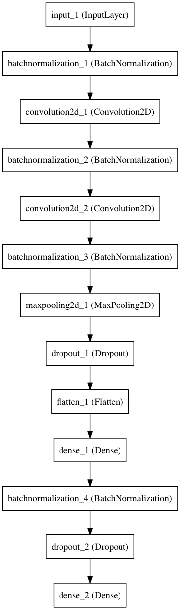
This discrepancy can be dealt with using the method of statistical ensembles — place one network and construct several copies of it with different initial values ​​and calculate their average result on the same input data. Here we will build three separate models. The differences between them can be easily represented in the form of a diagram, also constructed in Keras.

Core network

Ensemble

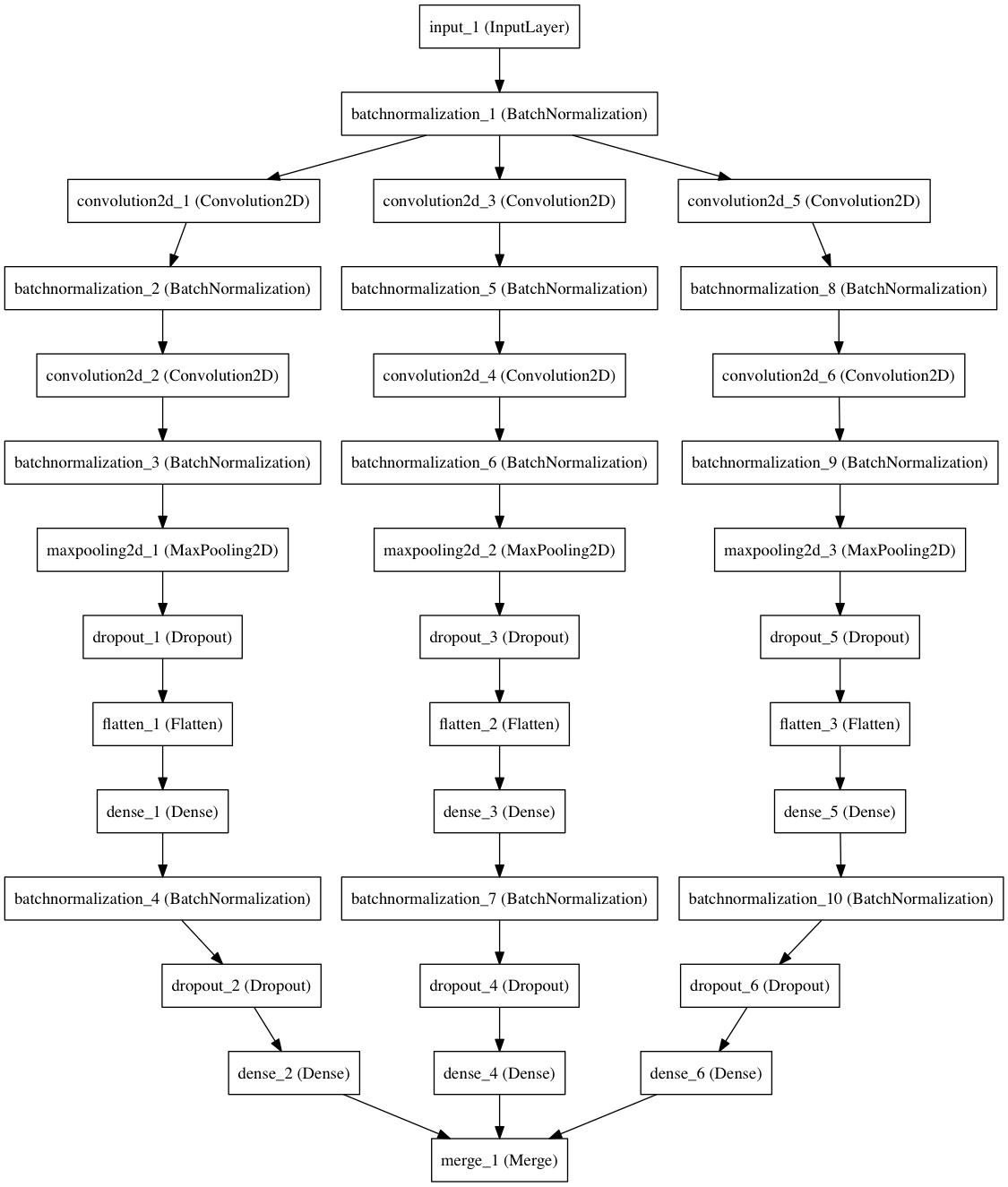
And again Keras allows you to carry out your plans by adding the minimum amount of code - we wrap up the method for constructing the component parts of the model in a cycle, combining their results in the last layer of merge .

 from keras.layers import merge # for merging predictions in an ensemble # ... ens_models = 3 # we will train three separate models on the data # ... inp_norm = BatchNormalization(axis=1)(inp) # Apply BN to the input (NB need to rename here) outs = [] # the list of ensemble outputs for i in range(ens_models): # conv_1 = Convolution2D(...)(inp_norm) # ... outs.append(Dense(num_classes, init='glorot_uniform', W_regularizer=l2(l2_lambda), activation='softmax')(drop)) # Output softmax layer out = merge(outs, mode='ave') # average the predictions to obtain the final output 

Early stopping

I will describe here another method as an introduction to a wider area of optimization of hyperparameters . So far, we have used the validation data set solely to monitor the progress of training, which is undoubtedly not rational (as this data is not used for constructive purposes). In fact, the validation set can serve as a basis for assessing network hyperparameters (such as depth, number of neurons / nuclei, regularization parameters, etc.). Imagine that a network is run with different combinations of hyperparameters, and then the decision is made based on their performance on the validation set. Please note that we do not need to know anything about the test set before we finally decide on the hyperparameters, because otherwise the signs of the test set will involuntarily join the learning process. This principle is also known as the golden rule of machine learning , and has been violated in many early approaches.

Perhaps the easiest way to use a validation set is to set the number of “ epochs ” (cycles) using a procedure known as early stop — just stop the learning process if over a given number of epochs (the patience parameter) losses do not begin to decrease. Since our data set is relatively small and saturated quickly, we will set the patience to five eras, and we will increase the maximum number of epochs to 50 (this number is unlikely to ever be reached).

The early stop mechanism is implemented in Keras through the EarlyStopping callback function class. Callbacks are called after each learning epoch using the callbacks parameter passed to the fit or fit_generator . As usual, everything is very compact: our program is increased only by one line of code.

 from keras.callbacks import EarlyStopping # ... num_epochs = 50 # we iterate at most fifty times over the entire training set # ... # fit the model on the batches generated by datagen.flow()---most parameters similar to model.fit model.fit_generator(datagen.flow(X_train, Y_train, batch_size=batch_size), samples_per_epoch=X_train.shape[0], nb_epoch=num_epochs, validation_data=(X_val, Y_val), verbose=1, callbacks=[EarlyStopping(monitor='val_loss', patience=5)]) # adding early stopping 

Just show me the code.

After applying the six optimization techniques described above, the code of our neural network will look like this.



99.47% , 99.12%. , , MNIST, . CIFAR-10, , .

: , , , , , , , ( 99.79% MNIST).

Conclusion

, :

-

-




, Keras, MNIST 90 .

. .

, , .

Thank!

Oh, and come to work with us? :)

wunderfund.io is a young foundation that deals with high-frequency algorithmic trading . High-frequency trading is a continuous competition of the best programmers and mathematicians of the whole world. By joining us, you will become part of this fascinating fight.

We offer interesting and challenging data analysis and low latency tasks for enthusiastic researchers and programmers. Flexible schedule and no bureaucracy, decisions are quickly made and implemented.

Join our team: wunderfund.io