Deep learning for newbies: recognizing images using convolutional networks

Introduction

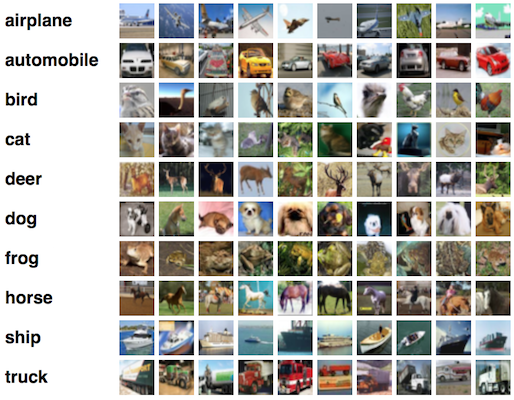
Introducing the second article in the series, conceived to help quickly understand the technology of deep learning ; we will move from basic principles to non-trivial features in order to get decent performance on two data sets: MNIST (handwritten classification) and CIFAR-10 (classification of small images into ten classes: airplane, car, bird, cat, deer, dog, frog , horse, ship and truck).

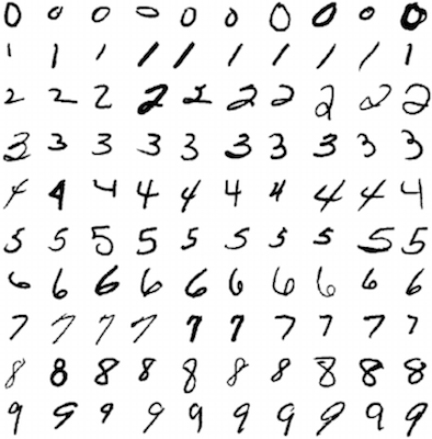
In the last lesson, we introduced the basic concepts of deep learning and showed how to quickly model neural network models using the Keras framework. Finally, a multilayer perceptron (MLP) containing two layers was applied to the MNIST, reaching an accuracy level of 98.2%, and this value is quite simple to improve. But nevertheless, a full-meshed perceptron is usually not chosen for tasks related to image recognition — in this case, it is much more common to take advantage of convolutional neural networks (CNN). Having completed this course, you will understand how it works and learn how to build CNN in Keras, achieving a good level of accuracy on CIFAR-10.

This article assumes familiarity with the previous article of the cycle .
')

Image processing

The above multilayer perceptron is the most powerful and possible neural networks of direct distribution. It consists of several layers, where each layer is organized in such a way that each neuron in one layer receives its copy of all the output data of the previous layer. This model is ideal for certain types of tasks, for example, training on a limited number of more or less unstructured parameters.

Nevertheless, let's see what happens with the number of parameters (weights) in such a model, when it receives raw data at the input. For example, CIFAR-10 contains 32 x 32 x 3 color images, and if we treat each channel of each pixel as an independent input parameter for the MLP, each neuron in the first hidden layer adds about 3000 new parameters to the model! And as the size of images grows, the situation quickly gets out of control, and this happens much earlier than the images reach the size that users of real applications usually work with.

One popular solution is to lower the resolution of images to the extent that MLP becomes applicable. However, when we simply lower the resolution, we risk losing a large amount of information, and it would be great if it was possible to carry out useful initial processing of information before applying the quality reduction without causing an explosive growth in the number of model parameters.

Convolution of functions

It turns out that there is a very effective way to solve this problem, which draws the image structure itself in our favor: it is assumed that the pixels that are close to each other “interact” more closely when forming the feature of interest to us than the pixels located in opposite corners. In addition, if in the process of classifying an image a small line is considered very important, it will not matter where the image is found.

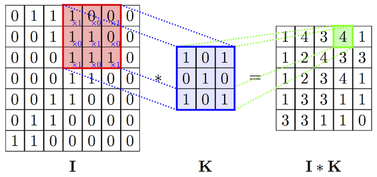
We introduce the concept of a convolution operator . Having a two-dimensional image I and a small matrix of K dimension $h \ times w$ (the so-called convolution kernel), constructed in such a way that graphically encodes any feature, we calculate the thumbnail image I * K , superimposing the core on the image in all possible ways and recording the sum of the products of the elements of the original image and the kernel:

$(I * K) _ {xy} = \ sum_ {i = 1} ^ h \ sum_ {j = 1} ^ wK_ {ij} \ times I_ {x + i-1, y + j-1}$

In fact, a precise definition implies that the core matrix will be transposed, but for machine learning tasks it does not matter whether this operation was performed or not.

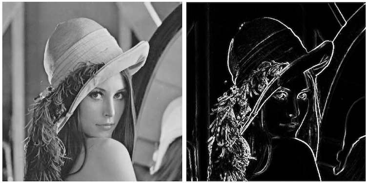
The figures below show the above formula schematically, and also show the result of applying the convolution operation (with two different cores) to the image in order to highlight the contours of the object.

Convolutional and downsampling layers

The convolution operator is the basis of the convolutional layer in CNN. The layer consists of a certain number of cores. $\ vec {K}$ (with additive offset components $\ vec {b}$ for each core) and calculates the convolution of the output image of the previous layer using each of the cores, each time adding an offset component. In the end, the activation function can be applied to the entire output image. $\ sigma$ . Usually, the input stream for a convolutional layer consists of d channels, for example, red / green / blue for the input layer, and in this case, the cores are also expanded in such a way that they also consist of d channels ; the following formula is obtained for one channel of the output image of a convolutional layer, where K is the core and b is the displacement component:

$\ textrm {conv} (I, K) _ {x, y} = \ sigma (b + \ sum_ {i = 1} ^ h \ sum_ {j = 1} ^ w \ sum_ {k = 1} ^ dK_ { ijk} \ times I_ {x + i-1, y + j-1, k})$

Note that since all we are doing here is adding and scaling the input pixels, the kernel can be obtained from the existing training set using the gradient descent method, similar to calculating weights in a multi-layer perceptron (MLP). In fact, the MLP could perfectly cope with the functions of the convolutional layer, but it would take much longer to train (as well as the training data).

Note also that the convolution operator is not at all limited to two-dimensional data: most deep learning frameworks (including Keras) provide layers for one-dimensional or three-dimensional convolution right out of the box.

It is also worth noting that although the convolutional layer reduces the number of parameters compared to a fully connected layer, it uses more hyperparameters — parameters that are chosen before the start of training.

In particular, the following hyperparameters are selected:

Depth - how many cores and displacement factors will be used in one layer;
The height ( height ) and width ( width ) of each core;
Step ( stride ) - how much the core shifts at each step when calculating the next pixel of the resulting image. Usually it is taken equal to 1, and the larger its value, the smaller the size of the output image;
Padding : note that convolving by any kernel of dimension more than 1x1 will reduce the size of the output image. Since in the general case it is desirable to preserve the size of the original image, the pattern is complemented with zeros at the edges.

As the reader has already guessed, convolution operations are not the only operations in CNN (although there are promising studies on the subject of “pure-ultra-precise” networks); they are more often used to isolate the most useful traits before downsampling and subsequent processing using MLP.

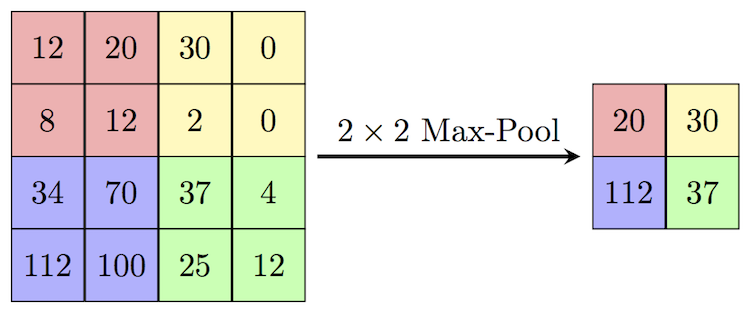
A popular way of downsampling an image is a subsample layer (also called a downsampling layer, in English, downsampling or pooling layer), which receives small separate image fragments (usually 2x2) as input and combines each fragment into one value. There are several possible ways of aggregation, most often the maximum is chosen from four pixels. This method is schematically shown below.

Total: regular CNN

Now that we have all the building blocks, let's look at what a normal CNN looks like in its entirety!

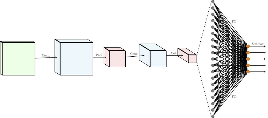
The usual CNN architecture for distributing images into k classes can be divided into two parts: a chain of alternating layers of convolution / subsample $\ textrm {Conv} \ to \ textrm {Pool}$ (sometimes with several layers of convolution in a row) and several fully connected layers (taking each pixel as an independent value) with a softmax layer as the final one. I’m not talking about activation functions here to make our scheme easier, but do not forget that after each convolutional or fully connected layer, an activation function, for example, ReLU, is usually applied after each convolutional or fully meshed layer.

One pass $\ textrm {Conv} \ to \ textrm {Pool}$ affects the image as follows: it reduces the length and width of a certain channel, but increases its value (depth).

Softmax and cross entropy were discussed in more detail in the previous lesson. Recall that the softmax function turns the vector of real numbers into a vector of probabilities (non-negative real numbers not exceeding 1). In our context, the output values are the probabilities of an image hitting a certain class. Minimizing the loss of cross-entropy provides confidence in determining whether an image belongs to a particular class, without taking into account the likelihood of other classes, thus, for softmax probabilistic problems, rather than, for example, the quadratic error method.

Retreat: retraining, regularization and dropout

For the first time (and, I hope, only once), I will draw your attention to the topic, at first glance, not related to the subject. It concerns a very important deep learning rock - the problem of retraining . Although this topic will be main in the next article of the cycle, the negative effect of retraining is noticeable on networks like the one we are going to build, which means you need to find a way to protect yourself from this phenomenon before we go any further. Fortunately, there is a very simple method that we apply.

Retraining is an unnecessarily precise correspondence of a neural network to a specific set of training examples in which the network loses its ability to generalize. In other words, our model could learn the training set (along with the noise that is present in it), but it could not recognize the hidden processes that generated this set. As an example, consider the problem of approximating a sinusoid with additive noise.

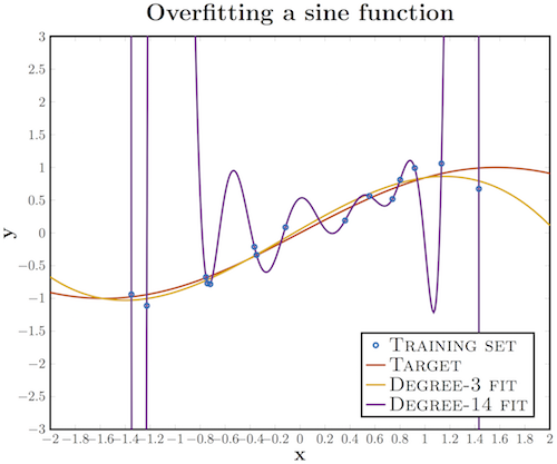
We have a training set (blue circles) obtained from the original sine curve, with some amount of noise. If we apply a third-degree polynomial to this data, we will get a good approximation of the original curve. Someone would argue that a 14th degree polynomial would fit better; Indeed, since we have 15 points, such an approximation would ideally describe the training set. However, in this case, the introduction of additional parameters into the model leads to catastrophic results: because our approximation takes noise into account, it does not coincide with the original curve anywhere except for the learning points.

Deep convolutional neural networks have a lot of different parameters, especially for fully connected layers. Re-training can manifest itself in the following form: if we do not have enough teaching examples, a small group of neurons can become responsible for most of the calculations, and the rest of the neurons will become redundant; or vice versa, some neurons can damage performance, while other neurons from their layer will not do anything except correcting their errors.

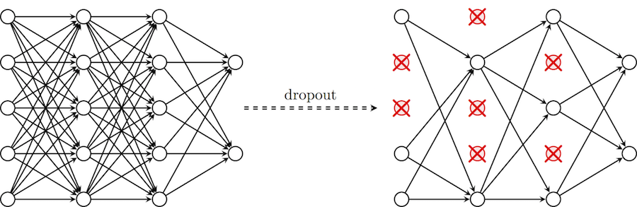
To help our network not to lose the ability to generalize in these circumstances, we introduce regularization techniques: instead of reducing the number of parameters, we impose restrictions on the model parameters during training, not allowing neurons to study the noise of training data. Here I will describe the dropout technique, which at first may seem “black magic”, but in fact helps to eliminate the situations described above. In particular, a dropout with the p parameter for one iteration of learning passes through all the neurons of a certain layer and with probability p completely excludes them from the network for the duration of the iteration . This will force the network to handle errors and not rely on the existence of a particular neuron (or group of neurons), but rather rely on the “consensus” of neurons within a single layer. This is a fairly simple method that effectively deals with the problem of retraining itself, without the need to introduce other regularizers. The diagram below illustrates this method.

Apply deep CNN to CIFAR-10

As a practical part, we construct a deep convolutional neural network and apply it to the classification of images from the CIFAR-10 set.

Imports are the same as last time , except that we use a greater variety of layers:

from keras.datasets import cifar10 # subroutines for fetching the CIFAR-10 dataset from keras.models import Model # basic class for specifying and training a neural network from keras.layers import Input, Convolution2D, MaxPooling2D, Dense, Dropout, Flatten from keras.utils import np_utils # utilities for one-hot encoding of ground truth values import numpy as np

 Using Theano backend.

As already mentioned, usually CNN uses more hyperparameters than MLP. In this guide, we will still use the previously known “good” values, but let's not forget that in the next lecture I will tell you how to choose them correctly.

We set the following hyperparameters:

batch_size - the number of training samples processed simultaneously in one iteration of the gradient descent algorithm;
num_epochs - the number of iterations of the learning algorithm over the entire training set;
kernel_size - kernel size in convolutional layers;
pool_size - subsample size in subsample layers;
onv_depth - the number of cores in the convolutional layers;
drop_prob (dropout probability) - we will apply dropout after each layer of the subsample, as well as after the fully connected layer;
hidden_size is the number of neurons in the full mesh layer of the MLP.

NB : I set 200 iterations, which can take too much time if you do not have a GPU (in this case convolutional layers will be the bottleneck). If you are going to train a network on a CPU, it’s worth reducing the number of iterations and / or cores.

 batch_size = 32 # in each iteration, we consider 32 training examples at once num_epochs = 200 # we iterate 200 times over the entire training set kernel_size = 3 # we will use 3x3 kernels throughout pool_size = 2 # we will use 2x2 pooling throughout conv_depth_1 = 32 # we will initially have 32 kernels per conv. layer... conv_depth_2 = 64 # ...switching to 64 after the first pooling layer drop_prob_1 = 0.25 # dropout after pooling with probability 0.25 drop_prob_2 = 0.5 # dropout in the FC layer with probability 0.5 hidden_size = 512 # the FC layer will have 512 neurons

Loading and preprocessing CIFAR-10 is exactly the same as loading and processing MNIST, where Keras performs everything automatically. The only difference is that now we do not consider each pixel as an independent input value, and therefore we do not transfer the image into one-dimensional space. We again convert the intensity of the pixels so that it falls into the interval [0,1] and use direct coding for the output values.

However, this time this stage will be performed for a more general case, which will make it easier to adapt to new data sets: the size will not be fixed, but calculated from the size of the data set, the number of classes will be determined by the number of unique labels in the training set, and normalization will be performed by dividing all elements by the maximum value of the training set.

NB : we also divide the test set by the maximum value of the training set, because our algorithms are not allowed to see the test data before the training process is completed, and therefore we cannot calculate any statistical metrics based on them except for applying the same transformations that occurred with a training set.

 (X_train, y_train), (X_test, y_test) = cifar10.load_data() # fetch CIFAR-10 data num_train, depth, height, width = X_train.shape # there are 50000 training examples in CIFAR-10 num_test = X_test.shape[0] # there are 10000 test examples in CIFAR-10 num_classes = np.unique(y_train).shape[0] # there are 10 image classes X_train = X_train.astype('float32') X_test = X_test.astype('float32') X_train /= np.max(X_train) # Normalise data to [0, 1] range X_test /= np.max(X_train) # Normalise data to [0, 1] range Y_train = np_utils.to_categorical(y_train, num_classes) # One-hot encode the labels Y_test = np_utils.to_categorical(y_test, num_classes) # One-hot encode the labels

It's time to simulate! Our network will consist of four layers of Convolution_2D and layers of MaxPooling2D after the second and fourth bundles. After the first subsample layer, we double the number of cores (along with the principle described above of sacrificing height and width to the depth). After that, the output image of the subsample layer is transformed into a one-dimensional vector (with the Flatten layer) and passes through two fully connected layers ( Dense ). On all layers, except for the output fully connected layer, the activation function ReLU is used, the last layer uses softmax.

To regularize our model, after each subsample layer and the first fully connected layer, a Dropout layer is applied. Here, Keras also stands out from the rest of the frameworks: it has an internal flag that automatically turns the dropout on and off, depending on whether the model is in the learning or testing phase.

For the rest, our model specification matches our previous settings for MNIST:

We use cross entropy as a function of loss;
We use Adam's optimizer for gradient descent;
We measure the accuracy of the model (since the source data is evenly divided into classes) *;
We leave 10% of the data for subsequent validation.

* To understand why accuracy is not suitable for cases when the distribution of data across classes is uneven, consider the limiting case when 90% of test data belongs to class x (for example, in a diagnostic task for patients with a rare disease). In this case, the classifier, which simply outputs x , reaches a significant accuracy of 90%, although in fact it does not perform either training or generalization.

 inp = Input(shape=(depth, height, width)) # NB depth goes first in Keras! # Conv [32] -> Conv [32] -> Pool (with dropout on the pooling layer) conv_1 = Convolution2D(conv_depth_1, kernel_size, kernel_size, border_mode='same', activation='relu')(inp) conv_2 = Convolution2D(conv_depth_1, kernel_size, kernel_size, border_mode='same', activation='relu')(conv_1) pool_1 = MaxPooling2D(pool_size=(pool_size, pool_size))(conv_2) drop_1 = Dropout(drop_prob_1)(pool_1) # Conv [64] -> Conv [64] -> Pool (with dropout on the pooling layer) conv_3 = Convolution2D(conv_depth_2, kernel_size, kernel_size, border_mode='same', activation='relu')(drop_1) conv_4 = Convolution2D(conv_depth_2, kernel_size, kernel_size, border_mode='same', activation='relu')(conv_3) pool_2 = MaxPooling2D(pool_size=(pool_size, pool_size))(conv_4) drop_2 = Dropout(drop_prob_1)(pool_2) # Now flatten to 1D, apply FC -> ReLU (with dropout) -> softmax flat = Flatten()(drop_2) hidden = Dense(hidden_size, activation='relu')(flat) drop_3 = Dropout(drop_prob_2)(hidden) out = Dense(num_classes, activation='softmax')(drop_3) model = Model(input=inp, output=out) # To define a model, just specify its input and output layers model.compile(loss='categorical_crossentropy', # using the cross-entropy loss function optimizer='adam', # using the Adam optimiser metrics=['accuracy']) # reporting the accuracy model.fit(X_train, Y_train, # Train the model using the training set... batch_size=batch_size, nb_epoch=num_epochs, verbose=1, validation_split=0.1) # ...holding out 10% of the data for validation model.evaluate(X_test, Y_test, verbose=1) # Evaluate the trained model on the test set!

View training listing

 Train on 45000 samples, validate on 5000 samples Epoch 1/200 45000/45000 [==============================] - 9s - loss: 1.5435 - acc: 0.4359 - val_loss: 1.2057 - val_acc: 0.5672 Epoch 2/200 45000/45000 [==============================] - 9s - loss: 1.1544 - acc: 0.5886 - val_loss: 0.9679 - val_acc: 0.6566 Epoch 3/200 45000/45000 [==============================] - 8s - loss: 1.0114 - acc: 0.6418 - val_loss: 0.8807 - val_acc: 0.6870 Epoch 4/200 45000/45000 [==============================] - 8s - loss: 0.9183 - acc: 0.6766 - val_loss: 0.7945 - val_acc: 0.7224 Epoch 5/200 45000/45000 [==============================] - 9s - loss: 0.8507 - acc: 0.6994 - val_loss: 0.7531 - val_acc: 0.7400 Epoch 6/200 45000/45000 [==============================] - 9s - loss: 0.8064 - acc: 0.7161 - val_loss: 0.7174 - val_acc: 0.7496 Epoch 7/200 45000/45000 [==============================] - 9s - loss: 0.7561 - acc: 0.7331 - val_loss: 0.7116 - val_acc: 0.7622 Epoch 8/200 45000/45000 [==============================] - 9s - loss: 0.7156 - acc: 0.7476 - val_loss: 0.6773 - val_acc: 0.7670 Epoch 9/200 45000/45000 [==============================] - 9s - loss: 0.6833 - acc: 0.7594 - val_loss: 0.6855 - val_acc: 0.7644 Epoch 10/200 45000/45000 [==============================] - 9s - loss: 0.6580 - acc: 0.7656 - val_loss: 0.6608 - val_acc: 0.7748 Epoch 11/200 45000/45000 [==============================] - 9s - loss: 0.6308 - acc: 0.7750 - val_loss: 0.6854 - val_acc: 0.7730 Epoch 12/200 45000/45000 [==============================] - 9s - loss: 0.6035 - acc: 0.7832 - val_loss: 0.6853 - val_acc: 0.7744 Epoch 13/200 45000/45000 [==============================] - 9s - loss: 0.5871 - acc: 0.7914 - val_loss: 0.6762 - val_acc: 0.7748 Epoch 14/200 45000/45000 [==============================] - 8s - loss: 0.5693 - acc: 0.8000 - val_loss: 0.6868 - val_acc: 0.7740 Epoch 15/200 45000/45000 [==============================] - 9s - loss: 0.5555 - acc: 0.8036 - val_loss: 0.6835 - val_acc: 0.7792 Epoch 16/200 45000/45000 [==============================] - 9s - loss: 0.5370 - acc: 0.8126 - val_loss: 0.6885 - val_acc: 0.7774 Epoch 17/200 45000/45000 [==============================] - 9s - loss: 0.5270 - acc: 0.8134 - val_loss: 0.6604 - val_acc: 0.7866 Epoch 18/200 45000/45000 [==============================] - 9s - loss: 0.5090 - acc: 0.8194 - val_loss: 0.6652 - val_acc: 0.7860 Epoch 19/200 45000/45000 [==============================] - 9s - loss: 0.5066 - acc: 0.8193 - val_loss: 0.6632 - val_acc: 0.7858 Epoch 20/200 45000/45000 [==============================] - 9s - loss: 0.4938 - acc: 0.8248 - val_loss: 0.6844 - val_acc: 0.7872 Epoch 21/200 45000/45000 [==============================] - 9s - loss: 0.4684 - acc: 0.8361 - val_loss: 0.6861 - val_acc: 0.7904 Epoch 22/200 45000/45000 [==============================] - 9s - loss: 0.4696 - acc: 0.8365 - val_loss: 0.6349 - val_acc: 0.7980 Epoch 23/200 45000/45000 [==============================] - 9s - loss: 0.4584 - acc: 0.8387 - val_loss: 0.6592 - val_acc: 0.7926 Epoch 24/200 45000/45000 [==============================] - 9s - loss: 0.4410 - acc: 0.8443 - val_loss: 0.6822 - val_acc: 0.7876 Epoch 25/200 45000/45000 [==============================] - 8s - loss: 0.4404 - acc: 0.8454 - val_loss: 0.7103 - val_acc: 0.7784 Epoch 26/200 45000/45000 [==============================] - 8s - loss: 0.4276 - acc: 0.8512 - val_loss: 0.6783 - val_acc: 0.7858 Epoch 27/200 45000/45000 [==============================] - 8s - loss: 0.4152 - acc: 0.8542 - val_loss: 0.6657 - val_acc: 0.7944 Epoch 28/200 45000/45000 [==============================] - 9s - loss: 0.4107 - acc: 0.8549 - val_loss: 0.6861 - val_acc: 0.7888 Epoch 29/200 45000/45000 [==============================] - 9s - loss: 0.4115 - acc: 0.8548 - val_loss: 0.6634 - val_acc: 0.7996 Epoch 30/200 45000/45000 [==============================] - 9s - loss: 0.4057 - acc: 0.8586 - val_loss: 0.7166 - val_acc: 0.7896 Epoch 31/200 45000/45000 [==============================] - 9s - loss: 0.3992 - acc: 0.8605 - val_loss: 0.6734 - val_acc: 0.7998 Epoch 32/200 45000/45000 [==============================] - 9s - loss: 0.3863 - acc: 0.8637 - val_loss: 0.7263 - val_acc: 0.7844 Epoch 33/200 45000/45000 [==============================] - 9s - loss: 0.3933 - acc: 0.8644 - val_loss: 0.6953 - val_acc: 0.7860 Epoch 34/200 45000/45000 [==============================] - 9s - loss: 0.3838 - acc: 0.8663 - val_loss: 0.7040 - val_acc: 0.7916 Epoch 35/200 45000/45000 [==============================] - 9s - loss: 0.3800 - acc: 0.8674 - val_loss: 0.7233 - val_acc: 0.7970 Epoch 36/200 45000/45000 [==============================] - 9s - loss: 0.3775 - acc: 0.8697 - val_loss: 0.7234 - val_acc: 0.7922 Epoch 37/200 45000/45000 [==============================] - 9s - loss: 0.3681 - acc: 0.8746 - val_loss: 0.6751 - val_acc: 0.7958 Epoch 38/200 45000/45000 [==============================] - 9s - loss: 0.3679 - acc: 0.8732 - val_loss: 0.7014 - val_acc: 0.7976 Epoch 39/200 45000/45000 [==============================] - 9s - loss: 0.3540 - acc: 0.8769 - val_loss: 0.6768 - val_acc: 0.8022 Epoch 40/200 45000/45000 [==============================] - 9s - loss: 0.3531 - acc: 0.8783 - val_loss: 0.7171 - val_acc: 0.7986 Epoch 41/200 45000/45000 [==============================] - 9s - loss: 0.3545 - acc: 0.8786 - val_loss: 0.7164 - val_acc: 0.7930 Epoch 42/200 45000/45000 [==============================] - 9s - loss: 0.3453 - acc: 0.8799 - val_loss: 0.7078 - val_acc: 0.7994 Epoch 43/200 45000/45000 [==============================] - 8s - loss: 0.3488 - acc: 0.8798 - val_loss: 0.7272 - val_acc: 0.7958 Epoch 44/200 45000/45000 [==============================] - 9s - loss: 0.3471 - acc: 0.8797 - val_loss: 0.7110 - val_acc: 0.7916 Epoch 45/200 45000/45000 [==============================] - 9s - loss: 0.3443 - acc: 0.8810 - val_loss: 0.7391 - val_acc: 0.7952 Epoch 46/200 45000/45000 [==============================] - 9s - loss: 0.3342 - acc: 0.8841 - val_loss: 0.7351 - val_acc: 0.7970 Epoch 47/200 45000/45000 [==============================] - 9s - loss: 0.3311 - acc: 0.8842 - val_loss: 0.7302 - val_acc: 0.8008 Epoch 48/200 45000/45000 [==============================] - 9s - loss: 0.3320 - acc: 0.8868 - val_loss: 0.7145 - val_acc: 0.8002 Epoch 49/200 45000/45000 [==============================] - 9s - loss: 0.3264 - acc: 0.8883 - val_loss: 0.7640 - val_acc: 0.7942 Epoch 50/200 45000/45000 [==============================] - 9s - loss: 0.3247 - acc: 0.8880 - val_loss: 0.7289 - val_acc: 0.7948 Epoch 51/200 45000/45000 [==============================] - 9s - loss: 0.3279 - acc: 0.8886 - val_loss: 0.7340 - val_acc: 0.7910 Epoch 52/200 45000/45000 [==============================] - 9s - loss: 0.3224 - acc: 0.8901 - val_loss: 0.7454 - val_acc: 0.7914 Epoch 53/200 45000/45000 [==============================] - 9s - loss: 0.3219 - acc: 0.8916 - val_loss: 0.7328 - val_acc: 0.8016 Epoch 54/200 45000/45000 [==============================] - 9s - loss: 0.3163 - acc: 0.8919 - val_loss: 0.7442 - val_acc: 0.7996 Epoch 55/200 45000/45000 [==============================] - 9s - loss: 0.3071 - acc: 0.8962 - val_loss: 0.7427 - val_acc: 0.7898 Epoch 56/200 45000/45000 [==============================] - 9s - loss: 0.3158 - acc: 0.8944 - val_loss: 0.7685 - val_acc: 0.7920 Epoch 57/200 45000/45000 [==============================] - 8s - loss: 0.3126 - acc: 0.8942 - val_loss: 0.7717 - val_acc: 0.8062 Epoch 58/200 45000/45000 [==============================] - 9s - loss: 0.3156 - acc: 0.8919 - val_loss: 0.6993 - val_acc: 0.7984 Epoch 59/200 45000/45000 [==============================] - 9s - loss: 0.3030 - acc: 0.8970 - val_loss: 0.7359 - val_acc: 0.8016 Epoch 60/200 45000/45000 [==============================] - 9s - loss: 0.3022 - acc: 0.8969 - val_loss: 0.7427 - val_acc: 0.7954 Epoch 61/200 45000/45000 [==============================] - 9s - loss: 0.3072 - acc: 0.8950 - val_loss: 0.7829 - val_acc: 0.7996 Epoch 62/200 45000/45000 [==============================] - 9s - loss: 0.2977 - acc: 0.8996 - val_loss: 0.8096 - val_acc: 0.7958 Epoch 63/200 45000/45000 [==============================] - 9s - loss: 0.3033 - acc: 0.8983 - val_loss: 0.7424 - val_acc: 0.7972 Epoch 64/200 45000/45000 [==============================] - 9s - loss: 0.2985 - acc: 0.9003 - val_loss: 0.7779 - val_acc: 0.7930 Epoch 65/200 45000/45000 [==============================] - 8s - loss: 0.2931 - acc: 0.9004 - val_loss: 0.7302 - val_acc: 0.8010 Epoch 66/200 45000/45000 [==============================] - 8s - loss: 0.2948 - acc: 0.8994 - val_loss: 0.7861 - val_acc: 0.7900 Epoch 67/200 45000/45000 [==============================] - 9s - loss: 0.2911 - acc: 0.9026 - val_loss: 0.7502 - val_acc: 0.7918 Epoch 68/200 45000/45000 [==============================] - 9s - loss: 0.2951 - acc: 0.9001 - val_loss: 0.7911 - val_acc: 0.7820 Epoch 69/200 45000/45000 [==============================] - 9s - loss: 0.2869 - acc: 0.9026 - val_loss: 0.8025 - val_acc: 0.8024 Epoch 70/200 45000/45000 [==============================] - 8s - loss: 0.2933 - acc: 0.9013 - val_loss: 0.7703 - val_acc: 0.7978 Epoch 71/200 45000/45000 [==============================] - 8s - loss: 0.2902 - acc: 0.9007 - val_loss: 0.7685 - val_acc: 0.7962 Epoch 72/200 45000/45000 [==============================] - 9s - loss: 0.2920 - acc: 0.9025 - val_loss: 0.7412 - val_acc: 0.7956 Epoch 73/200 45000/45000 [==============================] - 8s - loss: 0.2861 - acc: 0.9038 - val_loss: 0.7957 - val_acc: 0.8026 Epoch 74/200 45000/45000 [==============================] - 8s - loss: 0.2785 - acc: 0.9069 - val_loss: 0.7522 - val_acc: 0.8002 Epoch 75/200 45000/45000 [==============================] - 9s - loss: 0.2811 - acc: 0.9064 - val_loss: 0.8181 - val_acc: 0.7902 Epoch 76/200 45000/45000 [==============================] - 9s - loss: 0.2841 - acc: 0.9053 - val_loss: 0.7695 - val_acc: 0.7990 Epoch 77/200 45000/45000 [==============================] - 9s - loss: 0.2853 - acc: 0.9061 - val_loss: 0.7608 - val_acc: 0.7972 Epoch 78/200 45000/45000 [==============================] - 9s - loss: 0.2714 - acc: 0.9080 - val_loss: 0.7534 - val_acc: 0.8034 Epoch 79/200 45000/45000 [==============================] - 9s - loss: 0.2797 - acc: 0.9072 - val_loss: 0.7188 - val_acc: 0.7988 Epoch 80/200 45000/45000 [==============================] - 9s - loss: 0.2682 - acc: 0.9110 - val_loss: 0.7751 - val_acc: 0.7954 Epoch 81/200 45000/45000 [==============================] - 9s - loss: 0.2885 - acc: 0.9038 - val_loss: 0.7711 - val_acc: 0.8010 Epoch 82/200 45000/45000 [==============================] - 9s - loss: 0.2705 - acc: 0.9094 - val_loss: 0.7613 - val_acc: 0.8000 Epoch 83/200 45000/45000 [==============================] - 9s - loss: 0.2738 - acc: 0.9095 - val_loss: 0.8300 - val_acc: 0.7944 Epoch 84/200 45000/45000 [==============================] - 9s - loss: 0.2795 - acc: 0.9066 - val_loss: 0.8001 - val_acc: 0.7912 Epoch 85/200 45000/45000 [==============================] - 9s - loss: 0.2721 - acc: 0.9086 - val_loss: 0.7862 - val_acc: 0.8092 Epoch 86/200 45000/45000 [==============================] - 9s - loss: 0.2752 - acc: 0.9087 - val_loss: 0.7331 - val_acc: 0.7942 Epoch 87/200 45000/45000 [==============================] - 9s - loss: 0.2725 - acc: 0.9089 - val_loss: 0.7999 - val_acc: 0.7914 Epoch 88/200 45000/45000 [==============================] - 9s - loss: 0.2644 - acc: 0.9108 - val_loss: 0.7944 - val_acc: 0.7990 Epoch 89/200 45000/45000 [==============================] - 9s - loss: 0.2725 - acc: 0.9106 - val_loss: 0.7622 - val_acc: 0.8006 Epoch 90/200 45000/45000 [==============================] - 9s - loss: 0.2622 - acc: 0.9129 - val_loss: 0.8172 - val_acc: 0.7988 Epoch 91/200 45000/45000 [==============================] - 9s - loss: 0.2772 - acc: 0.9085 - val_loss: 0.8243 - val_acc: 0.8004 Epoch 92/200 45000/45000 [==============================] - 9s - loss: 0.2609 - acc: 0.9136 - val_loss: 0.7723 - val_acc: 0.7992 Epoch 93/200 45000/45000 [==============================] - 9s - loss: 0.2666 - acc: 0.9129 - val_loss: 0.8366 - val_acc: 0.7932 Epoch 94/200 45000/45000 [==============================] - 9s - loss: 0.2593 - acc: 0.9135 - val_loss: 0.8666 - val_acc: 0.7956 Epoch 95/200 45000/45000 [==============================] - 9s - loss: 0.2692 - acc: 0.9100 - val_loss: 0.8901 - val_acc: 0.7954 Epoch 96/200 45000/45000 [==============================] - 8s - loss: 0.2569 - acc: 0.9160 - val_loss: 0.8515 - val_acc: 0.8006 Epoch 97/200 45000/45000 [==============================] - 8s - loss: 0.2636 - acc: 0.9146 - val_loss: 0.8639 - val_acc: 0.7960 Epoch 98/200 45000/45000 [==============================] - 9s - loss: 0.2693 - acc: 0.9113 - val_loss: 0.7891 - val_acc: 0.7916 Epoch 99/200 45000/45000 [==============================] - 9s - loss: 0.2611 - acc: 0.9144 - val_loss: 0.8650 - val_acc: 0.7928 Epoch 100/200 45000/45000 [==============================] - 9s - loss: 0.2589 - acc: 0.9121 - val_loss: 0.8683 - val_acc: 0.7990 Epoch 101/200 45000/45000 [==============================] - 9s - loss: 0.2601 - acc: 0.9142 - val_loss: 0.9116 - val_acc: 0.8030 Epoch 102/200 45000/45000 [==============================] - 9s - loss: 0.2616 - acc: 0.9138 - val_loss: 0.8229 - val_acc: 0.7928 Epoch 103/200 45000/45000 [==============================] - 9s - loss: 0.2603 - acc: 0.9140 - val_loss: 0.8847 - val_acc: 0.7994 Epoch 104/200 45000/45000 [==============================] - 9s - loss: 0.2579 - acc: 0.9150 - val_loss: 0.9079 - val_acc: 0.8004 Epoch 105/200 45000/45000 [==============================] - 8s - loss: 0.2696 - acc: 0.9127 - val_loss: 0.7450 - val_acc: 0.8002 Epoch 106/200 45000/45000 [==============================] - 9s - loss: 0.2555 - acc: 0.9161 - val_loss: 0.8186 - val_acc: 0.7992 Epoch 107/200 45000/45000 [==============================] - 9s - loss: 0.2631 - acc: 0.9160 - val_loss: 0.8686 - val_acc: 0.7920 Epoch 108/200 45000/45000 [==============================] - 9s - loss: 0.2524 - acc: 0.9178 - val_loss: 0.9136 - val_acc: 0.7956 Epoch 109/200 45000/45000 [==============================] - 9s - loss: 0.2569 - acc: 0.9151 - val_loss: 0.8148 - val_acc: 0.7994 Epoch 110/200 45000/45000 [==============================] - 9s - loss: 0.2586 - acc: 0.9150 - val_loss: 0.8826 - val_acc: 0.7984 Epoch 111/200 45000/45000 [==============================] - 9s - loss: 0.2520 - acc: 0.9155 - val_loss: 0.8621 - val_acc: 0.7980 Epoch 112/200 45000/45000 [==============================] - 9s - loss: 0.2586 - acc: 0.9157 - val_loss: 0.8149 - val_acc: 0.8038 Epoch 113/200 45000/45000 [==============================] - 9s - loss: 0.2623 - acc: 0.9151 - val_loss: 0.8361 - val_acc: 0.7972 Epoch 114/200 45000/45000 [==============================] - 9s - loss: 0.2535 - acc: 0.9177 - val_loss: 0.8618 - val_acc: 0.7970 Epoch 115/200 45000/45000 [==============================] - 8s - loss: 0.2570 - acc: 0.9164 - val_loss: 0.7687 - val_acc: 0.8044 Epoch 116/200 45000/45000 [==============================] - 9s - loss: 0.2501 - acc: 0.9183 - val_loss: 0.8270 - val_acc: 0.7934 Epoch 117/200 45000/45000 [==============================] - 8s - loss: 0.2535 - acc: 0.9182 - val_loss: 0.7861 - val_acc: 0.7986 Epoch 118/200 45000/45000 [==============================] - 9s - loss: 0.2507 - acc: 0.9184 - val_loss: 0.8203 - val_acc: 0.7996 Epoch 119/200 45000/45000 [==============================] - 9s - loss: 0.2530 - acc: 0.9173 - val_loss: 0.8294 - val_acc: 0.7904 Epoch 120/200 45000/45000 [==============================] - 9s - loss: 0.2599 - acc: 0.9160 - val_loss: 0.8458 - val_acc: 0.7902 Epoch 121/200 45000/45000 [==============================] - 9s - loss: 0.2483 - acc: 0.9164 - val_loss: 0.7573 - val_acc: 0.7976 Epoch 122/200 45000/45000 [==============================] - 8s - loss: 0.2492 - acc: 0.9190 - val_loss: 0.8435 - val_acc: 0.8012 Epoch 123/200 45000/45000 [==============================] - 9s - loss: 0.2528 - acc: 0.9179 - val_loss: 0.8594 - val_acc: 0.7964 Epoch 124/200 45000/45000 [==============================] - 9s - loss: 0.2581 - acc: 0.9173 - val_loss: 0.9037 - val_acc: 0.7944 Epoch 125/200 45000/45000 [==============================] - 8s - loss: 0.2404 - acc: 0.9212 - val_loss: 0.7893 - val_acc: 0.7976 Epoch 126/200 45000/45000 [==============================] - 8s - loss: 0.2492 - acc: 0.9177 - val_loss: 0.8679 - val_acc: 0.7982 Epoch 127/200 45000/45000 [==============================] - 8s - loss: 0.2483 - acc: 0.9196 - val_loss: 0.8894 - val_acc: 0.7956 Epoch 128/200 45000/45000 [==============================] - 9s - loss: 0.2539 - acc: 0.9176 - val_loss: 0.8413 - val_acc: 0.8006 Epoch 129/200 45000/45000 [==============================] - 8s - loss: 0.2477 - acc: 0.9184 - val_loss: 0.8151 - val_acc: 0.7982 Epoch 130/200 45000/45000 [==============================] - 9s - loss: 0.2586 - acc: 0.9188 - val_loss: 0.8173 - val_acc: 0.7954 Epoch 131/200 45000/45000 [==============================] - 9s - loss: 0.2498 - acc: 0.9189 - val_loss: 0.8539 - val_acc: 0.7996 Epoch 132/200 45000/45000 [==============================] - 9s - loss: 0.2426 - acc: 0.9190 - val_loss: 0.8543 - val_acc: 0.7952 Epoch 133/200 45000/45000 [==============================] - 9s - loss: 0.2460 - acc: 0.9185 - val_loss: 0.8665 - val_acc: 0.8008 Epoch 134/200 45000/45000 [==============================] - 9s - loss: 0.2436 - acc: 0.9216 - val_loss: 0.8933 - val_acc: 0.7950 Epoch 135/200 45000/45000 [==============================] - 8s - loss: 0.2468 - acc: 0.9203 - val_loss: 0.8270 - val_acc: 0.7940 Epoch 136/200 45000/45000 [==============================] - 9s - loss: 0.2479 - acc: 0.9194 - val_loss: 0.8365 - val_acc: 0.8052 Epoch 137/200 45000/45000 [==============================] - 9s - loss: 0.2449 - acc: 0.9206 - val_loss: 0.7964 - val_acc: 0.8018 Epoch 138/200 45000/45000 [==============================] - 9s - loss: 0.2440 - acc: 0.9220 - val_loss: 0.8784 - val_acc: 0.7914 Epoch 139/200 45000/45000 [==============================] - 9s - loss: 0.2485 - acc: 0.9198 - val_loss: 0.8259 - val_acc: 0.7852 Epoch 140/200 45000/45000 [==============================] - 9s - loss: 0.2482 - acc: 0.9204 - val_loss: 0.8954 - val_acc: 0.7960 Epoch 141/200 45000/45000 [==============================] - 9s - loss: 0.2344 - acc: 0.9249 - val_loss: 0.8708 - val_acc: 0.7874 Epoch 142/200 45000/45000 [==============================] - 9s - loss: 0.2476 - acc: 0.9204 - val_loss: 0.9190 - val_acc: 0.7954 Epoch 143/200 45000/45000 [==============================] - 9s - loss: 0.2415 - acc: 0.9223 - val_loss: 0.9607 - val_acc: 0.7960 Epoch 144/200 45000/45000 [==============================] - 9s - loss: 0.2377 - acc: 0.9232 - val_loss: 0.8987 - val_acc: 0.7970 Epoch 145/200 45000/45000 [==============================] - 9s - loss: 0.2481 - acc: 0.9201 - val_loss: 0.8611 - val_acc: 0.8048 Epoch 146/200 45000/45000 [==============================] - 9s - loss: 0.2504 - acc: 0.9197 - val_loss: 0.8411 - val_acc: 0.7938 Epoch 147/200 45000/45000 [==============================] - 9s - loss: 0.2450 - acc: 0.9216 - val_loss: 0.7839 - val_acc: 0.8028 Epoch 148/200 45000/45000 [==============================] - 9s - loss: 0.2327 - acc: 0.9250 - val_loss: 0.8910 - val_acc: 0.8054 Epoch 149/200 45000/45000 [==============================] - 9s - loss: 0.2432 - acc: 0.9219 - val_loss: 0.8568 - val_acc: 0.8000 Epoch 150/200 45000/45000 [==============================] - 9s - loss: 0.2436 - acc: 0.9236 - val_loss: 0.9061 - val_acc: 0.7938 Epoch 151/200 45000/45000 [==============================] - 9s - loss: 0.2434 - acc: 0.9222 - val_loss: 0.8439 - val_acc: 0.7986 Epoch 152/200 45000/45000 [==============================] - 9s - loss: 0.2439 - acc: 0.9225 - val_loss: 0.9002 - val_acc: 0.7994 Epoch 153/200 45000/45000 [==============================] - 8s - loss: 0.2373 - acc: 0.9237 - val_loss: 0.8756 - val_acc: 0.7880 Epoch 154/200 45000/45000 [==============================] - 8s - loss: 0.2359 - acc: 0.9238 - val_loss: 0.8514 - val_acc: 0.7936 Epoch 155/200 45000/45000 [==============================] - 9s - loss: 0.2435 - acc: 0.9222 - val_loss: 0.8377 - val_acc: 0.8080 Epoch 156/200 45000/45000 [==============================] - 9s - loss: 0.2478 - acc: 0.9204 - val_loss: 0.8831 - val_acc: 0.7992 Epoch 157/200 45000/45000 [==============================] - 9s - loss: 0.2337 - acc: 0.9253 - val_loss: 0.8453 - val_acc: 0.7994 Epoch 158/200 45000/45000 [==============================] - 9s - loss: 0.2336 - acc: 0.9257 - val_loss: 0.9027 - val_acc: 0.7882 Epoch 159/200 45000/45000 [==============================] - 9s - loss: 0.2384 - acc: 0.9230 - val_loss: 0.9121 - val_acc: 0.8016 Epoch 160/200 45000/45000 [==============================] - 9s - loss: 0.2481 - acc: 0.9217 - val_loss: 0.9495 - val_acc: 0.7974 Epoch 161/200 45000/45000 [==============================] - 9s - loss: 0.2450 - acc: 0.9224 - val_loss: 0.8510 - val_acc: 0.7884 Epoch 162/200 45000/45000 [==============================] - 9s - loss: 0.2433 - acc: 0.9220 - val_loss: 0.8979 - val_acc: 0.7948 Epoch 163/200 45000/45000 [==============================] - 9s - loss: 0.2339 - acc: 0.9262 - val_loss: 0.8979 - val_acc: 0.7978 Epoch 164/200 45000/45000 [==============================] - 9s - loss: 0.2298 - acc: 0.9257 - val_loss: 0.9036 - val_acc: 0.7990 Epoch 165/200 45000/45000 [==============================] - 9s - loss: 0.2404 - acc: 0.9236 - val_loss: 0.8341 - val_acc: 0.8052 Epoch 166/200 45000/45000 [==============================] - 9s - loss: 0.2402 - acc: 0.9227 - val_loss: 0.8731 - val_acc: 0.7996 Epoch 167/200 45000/45000 [==============================] - 9s - loss: 0.2367 - acc: 0.9250 - val_loss: 0.9218 - val_acc: 0.7992 Epoch 168/200 45000/45000 [==============================] - 9s - loss: 0.2267 - acc: 0.9262 - val_loss: 0.8767 - val_acc: 0.7922 Epoch 169/200 45000/45000 [==============================] - 9s - loss: 0.2336 - acc: 0.9254 - val_loss: 0.8418 - val_acc: 0.8038 Epoch 170/200 45000/45000 [==============================] - 9s - loss: 0.2434 - acc: 0.9232 - val_loss: 0.8362 - val_acc: 0.7920 Epoch 171/200 45000/45000 [==============================] - 9s - loss: 0.2328 - acc: 0.9265 - val_loss: 0.8712 - val_acc: 0.7950 Epoch 172/200 45000/45000 [==============================] - 9s - loss: 0.2346 - acc: 0.9262 - val_loss: 0.9256 - val_acc: 0.7976 Epoch 173/200 45000/45000 [==============================] - 8s - loss: 0.2382 - acc: 0.9242 - val_loss: 0.8875 - val_acc: 0.7982 Epoch 174/200 45000/45000 [==============================] - 9s - loss: 0.2400 - acc: 0.9239 - val_loss: 0.8264 - val_acc: 0.7864 Epoch 175/200 45000/45000 [==============================] - 9s - loss: 0.2334 - acc: 0.9261 - val_loss: 0.9178 - val_acc: 0.8014 Epoch 176/200 45000/45000 [==============================] - 9s - loss: 0.2427 - acc: 0.9219 - val_loss: 0.8458 - val_acc: 0.7920 Epoch 177/200 45000/45000 [==============================] - 9s - loss: 0.2310 - acc: 0.9257 - val_loss: 0.9171 - val_acc: 0.8062 Epoch 178/200 45000/45000 [==============================] - 9s - loss: 0.2310 - acc: 0.9265 - val_loss: 0.8544 - val_acc: 0.7990 Epoch 179/200 45000/45000 [==============================] - 9s - loss: 0.2378 - acc: 0.9240 - val_loss: 0.9259 - val_acc: 0.8000 Epoch 180/200 45000/45000 [==============================] - 9s - loss: 0.2381 - acc: 0.9242 - val_loss: 0.8573 - val_acc: 0.8056 Epoch 181/200 45000/45000 [==============================] - 9s - loss: 0.2231 - acc: 0.9297 - val_loss: 0.8935 - val_acc: 0.8002 Epoch 182/200 45000/45000 [==============================] - 9s - loss: 0.2419 - acc: 0.9248 - val_loss: 1.0145 - val_acc: 0.7900 Epoch 183/200 45000/45000 [==============================] - 9s - loss: 0.2336 - acc: 0.9266 - val_loss: 0.8838 - val_acc: 0.8006 Epoch 184/200 45000/45000 [==============================] - 9s - loss: 0.2429 - acc: 0.9242 - val_loss: 0.8685 - val_acc: 0.7918 Epoch 185/200 45000/45000 [==============================] - 9s - loss: 0.2317 - acc: 0.9260 - val_loss: 0.8297 - val_acc: 0.7942 Epoch 186/200 45000/45000 [==============================] - 9s - loss: 0.2330 - acc: 0.9264 - val_loss: 0.8831 - val_acc: 0.8026 Epoch 187/200 45000/45000 [==============================] - 9s - loss: 0.2353 - acc: 0.9254 - val_loss: 0.8934 - val_acc: 0.7956 Epoch 188/200 45000/45000 [==============================] - 9s - loss: 0.2312 - acc: 0.9247 - val_loss: 0.9275 - val_acc: 0.8042 Epoch 189/200 45000/45000 [==============================] - 9s - loss: 0.2239 - acc: 0.9282 - val_loss: 0.9246 - val_acc: 0.7934 Epoch 190/200 45000/45000 [==============================] - 9s - loss: 0.2349 - acc: 0.9253 - val_loss: 0.8628 - val_acc: 0.8000 Epoch 191/200 45000/45000 [==============================] - 9s - loss: 0.2313 - acc: 0.9266 - val_loss: 0.9020 - val_acc: 0.7978 Epoch 192/200 45000/45000 [==============================] - 9s - loss: 0.2358 - acc: 0.9254 - val_loss: 0.9481 - val_acc: 0.7966 Epoch 193/200 45000/45000 [==============================] - 9s - loss: 0.2298 - acc: 0.9276 - val_loss: 0.8791 - val_acc: 0.8010 Epoch 194/200 45000/45000 [==============================] - 9s - loss: 0.2279 - acc: 0.9265 - val_loss: 0.8890 - val_acc: 0.7976 Epoch 195/200 45000/45000 [==============================] - 9s - loss: 0.2330 - acc: 0.9273 - val_loss: 0.8893 - val_acc: 0.7890 Epoch 196/200 45000/45000 [==============================] - 9s - loss: 0.2416 - acc: 0.9243 - val_loss: 0.9002 - val_acc: 0.7922 Epoch 197/200 45000/45000 [==============================] - 9s - loss: 0.2309 - acc: 0.9273 - val_loss: 0.9232 - val_acc: 0.7990 Epoch 198/200 45000/45000 [==============================] - 9s - loss: 0.2247 - acc: 0.9278 - val_loss: 0.9474 - val_acc: 0.7980 Epoch 199/200 45000/45000 [==============================] - 9s - loss: 0.2335 - acc: 0.9256 - val_loss: 0.9177 - val_acc: 0.8000 Epoch 200/200 45000/45000 [==============================] - 9s - loss: 0.2378 - acc: 0.9254 - val_loss: 0.9205 - val_acc: 0.7966 9984/10000 [============================>.] - ETA: 0s [0.97292723369598388, 0.7853]

76.6% ; , 90%, , . , 96.53%.

, , , . , MNIST ; CNN dropout' 99.3%.

Conclusion

, , ( , dropout), CNN Keras, CIFAR-10 50 .

, , , .

Source: https://habr.com/ru/post/314872/

All Articles