Build a Voronoi diagram by 'divide and conquer'. Lloyd's Relaxation

Recently, an article devoted entirely to Voronoi diagrams was published on Habrahabr. In the article, the author describes the Forchun algorithm in detail, which is used to construct the Voronoi diagram for O (n * log (n)) . It is worth noting that the description of this algorithm more than once appeared in runet, while other algorithms (with the same asymptotics) are told absolutely nothing. This article corrects this misunderstanding , and is also a great addition to the previously published material.
Below I will talk about the 'divide and conquer' algorithm for constructing a Voronoi diagram for O (n * log (n)) , as well as, based on my practical experience, about really cool things in which this applies. In general, divide-and-conquer algorithms are a kind of programming classic (I think every programmer heard about this sorting method), are well parallelized and easy to read (unless, of course, you know the basic idea of the algorithm).
Description of the 'divide and conquer' algorithm for constructing the Voronoi diagram
The initial set of points is sorted by one of the coordinates (we assume, x) and is divided into two, approximately equal sets. Each of the sets obtained is again divided into two, and this happens until no more than two points remain in each of the sets. It is easy to see that such partitions will be no more than log (n) . Further, for each obtained set, Voronoi diagrams are constructed, after which, in the reverse order of division, these diagrams are combined into one. The resulting Voronoi diagram will be the final result.
In order for the described algorithm to have complexity of order O (n * log (n)) , it is necessary to perform the process of combining two Voronoi diagrams for O (N) . I note that for a set of two points, the Voronoi diagram will be the median perpendicular of the segment formed by these two points.
')
Suppose that all points are sorted by X coordinate, and the initial set is divided into two, and for each one a Voronoi diagram is constructed. Perform the union of these sets and their diagrams as follows:
⦁ 1. For each of the subsets we find a convex hull (note that the construction of a convex hull for each of the sets can be done in the same 'divide and conquer' : that is, at each step of combining the Voronoi diagrams we combine the convex hulls of these sets in O (N) ).
⦁ 2. Now that we have two convex hulls of the original sets, we find the 'upper and lower' boundaries of these sets: that is, we have to find two such segments that combine the two convex hulls into one (naturally, convex). Thus, we fulfill the conditions of step 1, and also get the initialization values for step 3. This step, as I wrote, can be performed in O (N) .
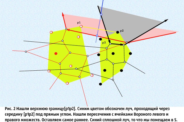
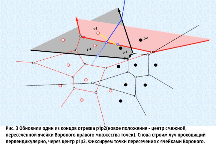
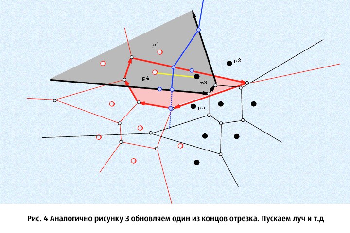
⦁ 3. From the obtained segments in step 2 , we choose any and denote by L (the remaining denote by Q ), and through its middle, let us perpendicularly an infinite ray. Imagine that a given ray only enters the original set, and find its intersections with the cells of the Voronoi diagrams of the original sets (it is believed that the ray extends forward, that is, it has a direction). We intersect the beam only with those Voronoi cells, whose centers are the ends of the segment, perpendicular to which we let the beam. We need to find the point of intersection of the beam with the corresponding Voronoi cells and choose among them the one that intersects earlier. We denote this point by M , and the cell we crossed will be remembered and denoted by V. Next, we will do the following: leave the end of the segment L , which is the center for a non-intersected Voronoi cell, alone, but the one that was the center of the cell we crossed is updating: we crossed one of the sides of the Voronoi cell, then the new end of the segment L will be center of the Voronoi cell adjacent on this side with a crossed cell. In the special set S (the boundary of two Voronoi diagrams is stored in it), we must add the part of the ray that extends to the intersection with the side of the cell. Repeat step 3 until the values of the ends of the segment L become equal to the values of the ends of the segment Q. As a result, in the set S there will be a continuous broken ray. The proof of many facts presented here (for example, the continuity of a ray in the set S ) can be found in [1] .
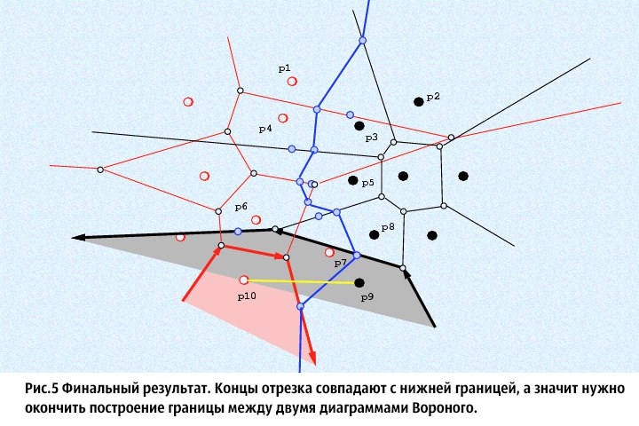
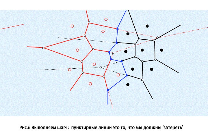
⦁ 4. We obtained the set S , which is a continuous broken ray. This ray is the boundary connecting the Voronoi diagrams of the two sets. To obtain the final result, it is necessary for the Voronoi diagram of the left set to “wipe” those segments that are to the right of the received beam, and for the Voronoi diagram of the right set to “wipe” those that are to the left. To do this quickly is not a problem: when we cross a cell with a beam, it is obvious that the beam will first enter it, and then, at some specific moment, it will come out. We need to 'catch' these events, and depending on which diagram of the set we are working (left or right), remove the left or right chain of edges of the Voronoi cell, which we crossed with a beam, and add the necessary part from the set S to it .
The algorithm described above is difficult to understand without a good illustration (the pictures were taken here ):

Well, I will finish this subsection of the publication on the fact that if the points have the same X coordinate, then it is worthwhile to sort them according to the Y coordinate, so that they are evenly and consistently divided.
Application of the Voronoi Diagrams - Lloyd's Relaxation
Lloyd's Relaxation is one of the amazing and 'sticky' algorithms that actively uses Voronoi diagrams. I will describe the algorithm itself:
⦁ 1. We construct the Voronoi diagram for the initial set of points, form Voronoi cells.
⦁ 2. Find the “Center Mass” of each Voronoi cell (the sum of the coordinates of the Voronoi cell vertices divided by their number).
⦁ 3. Shift the center of each Voronoi cell to the position of the calculated “Center Mass”.
⦁ 4. We repeat this procedure N times: until the shift distance is close to zero.
What do we get in the end? The result can be seen on these two short videos:
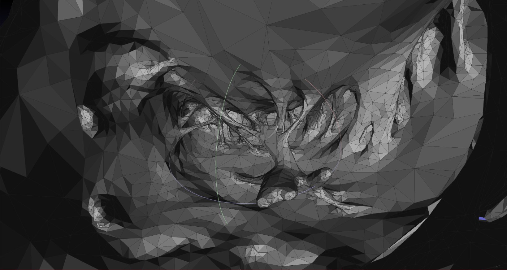
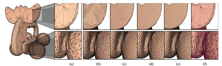
It looks beautiful, but a bit useless !? Far away! In my practical experience, Lloyd’s relaxation was applied in 3D modeling: in the so-called “mesh remeshing” . That is, the grid is given (usually after processing by a cheap Chinese scanner) and the task is to turn the resulting 'jumble' of triangles into something beautiful and alive: into something that can be used for more or less accurate calculations (calculation of 'grid curvature', approximation of triangulation points). grids with infinitely smooth surfaces, etc.), trying not to deviate much from the original “scanner” mesh (moreover, this accuracy is set by the user, and this “remixing” is called adaptive). There is also uniform “remixing” ( uniform) - here, it is not the deviation that is set, but the desired edge length in the triangle). I spoke a little and forgot to explain what we mean by the word 'beautiful' grid. A grid is called 'beautiful' if its structure consists mainly of equilateral triangles, and the valency of each vertex at such a grid is 6 (if the vertex is internal, well, i.e. 360. / 6. = 60 deg. - degree of angle of an equilateral triangle) or 4 (if the vertex lies on an open edge, that is, the triangles with this vertex 3). Well, one of the important stages of obtaining such a grid is the construction of the Voronoi diagram and the use of Lloyd's relaxation. Actually, we get something in this spirit (neatly, the pictures are big!):
Pictures of the result of the work of 'remiching', coded by me
Before:
After:
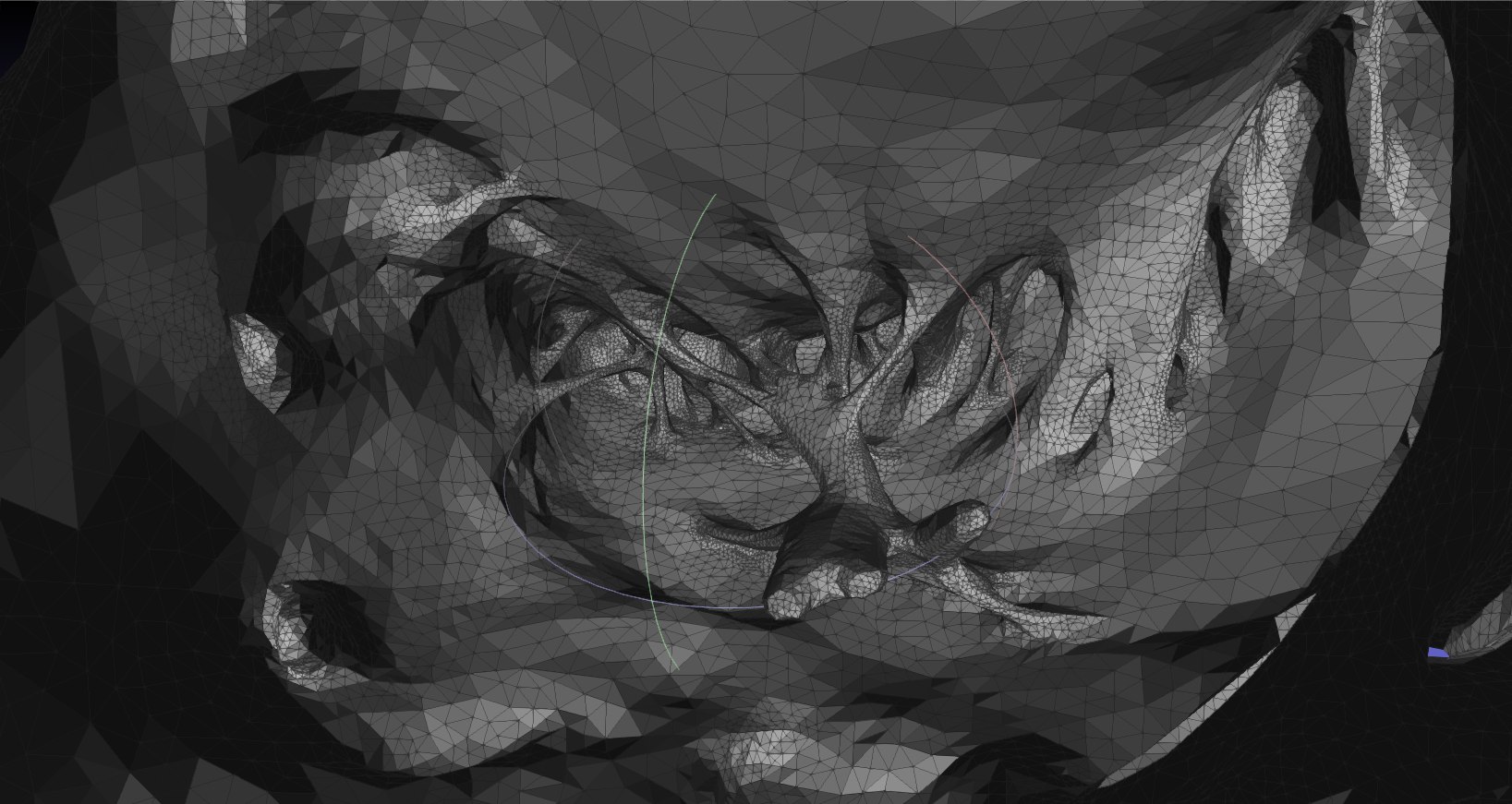
And now before and after in one image:
By the way, you can see that the original was obtained using the Marching Cubes algorithm.
After:
And now before and after in one image:
By the way, you can see that the original was obtained using the Marching Cubes algorithm.
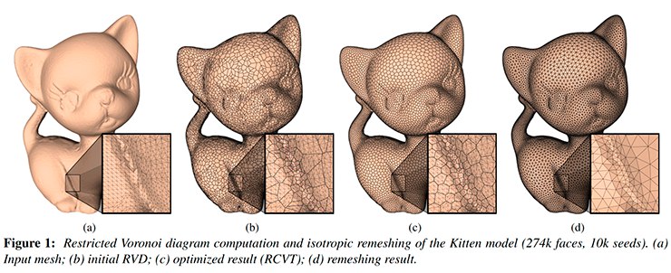
Well, the pictures are smaller, but from the Internet:
And ... (where can it be without it) - the statue of David:
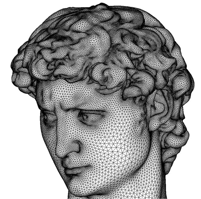
Beauty, and only!
I would like to conclude that using the Lloyd's algorithm is a costly business. And to obtain a faster result, without much loss in quality, so-called 'Energy Minimization' methods were developed. You can read in [2]
Useful links and literature
[0] Cool article on Habrahabr about Voronoi diagrams
[1] The original description of the algorithm, with all the evidence.
[2] Comparison of Energy Minimization Methods
[3] A short article on the "Divide and Conquer" Voronoi diagram construction algorithm.
Source: https://habr.com/ru/post/314852/
All Articles