Formulation of the problem

There is a DC motor. The task is to develop, assemble and test a device that allows realizing the current loop as applied to this engine. The desired transition time on a locked engine (without back-EMF) is no more than 10 ms. Interface communication with an external control controller - SPI.



DC motor, collector, maximum voltage 24V, operating current up to 5A.



What does current loop mean? The most common drivers for engine control are all kinds of half-bridge variations that increase the voltage. And I want the driver to take at the input not the voltage, but the amperage. The force developed by the electric drive is directly proportional to the strength of the flowing current. So, it is directly proportional to the acceleration on the motor shaft. Such a current loop will avoid the perversions that need to be done without it, as I did here .

')

I have broken this text into two articles:

• 1. Measurement of motor resistance and inductance
• 2. Development of the control circuit

This is how the layout of the controlling iron looks like:

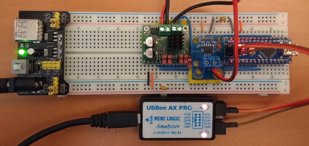
Iron

The system will include:

• The power chip of the keys, which takes the input PWM signal and amplifies it.
• Current sensor.
• Control microcontroller that implements feedback and control law.

Power driver

The widely available board ($ 18) from Pololu based on the Freescale MC33926 chip, the maximum PWM frequency of 20kHz, 5A at the peak, and the switching voltage from 5 to 28 volts was chosen as the power driver.



This chip was taken for its ability to measure the absolute magnitude of the flowing current, which in the end was not used. Thus, you can save a little by taking a cheaper driver with similar characteristics.

Current sensor and its verification

The Allegro ACS714 Hall sensor ($ 3) is selected as the current sensor , which produces an analog signal with a center of 2.5V and 185mV / A, a typical error of 1.5%. An RC-chain was added to the sensor as a low-pass filter with a cut-off frequency of 16 kHz.



The current sensor was powered from a 4.96V source, a resistor was connected in series with the sensor, through which 2A was passed. The theoretical voltage at the output pin should be 4.96 / 2 + (2 * 0.185 + - 1.5%), the measurement showed 2.84 V, which fits into the calculated parameters. Then the direction of current flow through the resistor was varied, at -2A, the measured voltage at the output pin of the sensor was 2.11V, which again fits into the calculated parameters:







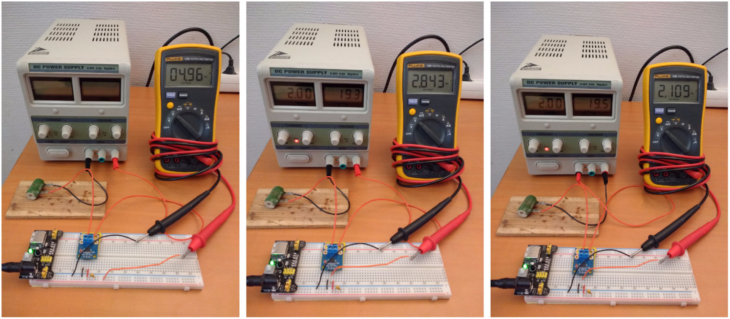
This check was necessary because I bought several prototypes with ACS712 and ACS714 from different manufacturers, and only one got into the datasheet parameters!

Microcontroller

ATMega328p operating at 16 MHz was chosen as the control microcontroller. The binding of the microcontroller is a Chinese clone Arduino Nano v3 ($ 1.5).



The microcontroller generates a PWM signal through an eight-bit counter with a divider 8, thus the frequency of the PWM signal is 16 * 10 ^ 6/255/8 = 7.8 kHz, which fits into the maximum available for the 20kHz driver.



The ADC divider of the microcontroller is set to 128; since each measurement requires approximately 13 clocks, the maximum measurement frequency of the flowing current is approximately 16 * 10 ^ 6/128/13 = 9.6 kHz. Measurements are performed in the background, notifying the main program of the termination by calling the appropriate interrupt.

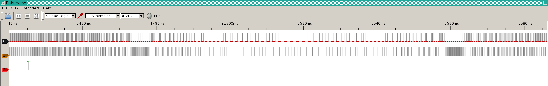
Logs

I have long struggled with how to record what is happening inside the microcontroller, because he has very little memory. As a result, I found that the native SPI interface is very fast, and as a result, all debugging information is transmitted by the microcontroller via the SPI interface, the widely available ( $ 10 on dilextreme , $ 6 on aliexpress) Chinese clone of the logic analyzer Saelae Pro 8 Logic was used to record it. After a completely uncomplicated manipulation of the VID / PID flashing , it can be used with the native software from Saelae. I use sigrok (pulseview). It has an exceptionally simple format of log files, which I just read with my own handwritten program in fifty lines. I bought this analyzer on the advice of gbg , which I remotely repaired my Spectrum (thank you so much!), And I consider this the most profitable investment in the last two years.



For example, I gave a sinusoidal signal (in PWM) to the controller output, and the logic analyzer sees it perfectly:







All this was combined together, the photo is given in the title of the post.

Lyrical digression

Almost all the articles that I post here are my work diary. I learn something (in this case, control theory) and carefully write down what I learned. The best way to write is to write an explanation of how this all works. Then I post articles at various sites, for example here.



I have two goals when writing text:



a) get feedback from people who know more than me. For example, almost everything that I learned for these two articles, I was told by the distinguished Arastas , I ask you to love and favor: a person who spends personal time learning such obtuses like me.



Again, gbg , who wrote me linear algebra for my lectures on computer graphics , and then for many thousands of kilometers by telephone debugil me electronics.



b) just write it down: this way I get a library of personal experience, which I periodically return to. By the way, themed media, what percentage of authors agree to your terms of support program?

Required educational program

Fourier transform

The first thing to understand when reading my texts: I believe that function and vector are one and the same. All the talk about infinity bored me and obscure the essence of what is happening. Generalized functions and the like are a way to treat pathological cases using the same language as cases where there are no pathologies. Here only pathologies do not interest me.



Valery Opoytsev (Boss) spoke well on this subject:

In any field it is useful to be in a suitable environment of oral communication, where the husks of a book fall off. There sometimes nothing changes in essence, but there is a feeling of falling into a rut and liberation from dogma. For science, which is always in a mask, this is especially important. The essence behind the scenes, before the eyes - lace. And forever something is missing. That simplicity, the complexity, but just can not determine - what. Something is striding somewhere, you are on the side of the road, and time goes into the sand, not to mention life.



Next, an attempt is made to move the situation from the scene, simulating a written environment where “the covers fall down”. The external outline of the content is more or less unclear from the table of contents, but the main goal is the one behind the scenes. Remove the veil, make-up, remove the scenery. To oversimplify, even to lie a little, for the dosing of truth is the cornerstone of explanation. The results, overloaded with details, do not crawl where necessary. Illumination happens when a plump head falls to the level of “two and two”, while the bill goes to the millions. Such is the dialectic here.

If we have a vector (7,12,18, -2), then it can be considered as a set of coefficients in a weighted sum. 7 * (1,0,0,0) + 12 * (0,1,0,0) + 18 * (0,0,1,0) + (-2) * (0,0,0,1) . Exactly the same can be considered this vector as function values ​​at points 0, 1, 2, 3, because our vectors (0,1,0,0) and others like it can be considered as a shift of a single impulse:





If we constantly increase the number of vectors (shifted unit impulses) in the basis, we get the usual functions.



Unfortunately, it is rather inconvenient to work with such a basis. Let's take the following function as an example:





We have already talked about what Fourier transform is. In short, this is a change of basis.



In our case, the Fourier transform is a function from real to complex numbers:





The function argument (real number) is simply the number of the basis function or vector (in fact, a pair of basis functions), and its value is the corresponding (pair) of coordinates in for these two vectors in the basis. The Fourier basis is the sines and cosines of various frequencies. Frequency is the number of the basis function.



For our particular function f (t), which is already a weighted sum of sine and cosine, it is very easy to calculate its decomposition into the Fourier basis:





That is, our function f (t) has zero coordinates for all basis vectors, except vectors number 11 and 41.



How is the Fourier basis useful? For example, the operation of differentiation linearly transforms this basis. Suppose we want to calculate the Fourier transform of the derivative f '(t). How to do it? Alternatively, in the forehead: first calculate the derivative, and then calculate the Fourier transform:





Obviously, when differentiating sin (x), it becomes sin (x + 90 °), that is, it is extremely easy to find a correspondence expansion in the Fourier basis of the original function and its derivative:





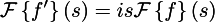
Multiplication by i is simply a rotation of the complex plane, which corresponds to + 90 ° in the argument of our function. That is, the operation of differentiation, which is difficult to do in the basis of single impulses, in the Fourier basis is just a scaling and a rotation of 90 degrees. Beautiful, is not it?

Laplace transform

Roughly the same story happens with the Laplace transform. Unfortunately, unlike the Fourier basis, the Laplace basis is non-orthogonal, so for an intuitive understanding a bit more complicated. Well, not the essence. Laplace went a little further. If Fourier had only sinusoids in the basis, then Laplace had an exponential decay in the basis of the sinusoids. Where did he get them? This is extremely, extremely useful in solving linear differential equations. Let's think about what function transforms itself into differentiation? Exhibitor. And when differentiating twice? Sinus. And their combinations provide all the possible functions that may appear when solving (linear) diffuros, which was used by the Marquis de Laplace.



We will not go into details of how these properties are derived (better consider carefully the properties of the Fourier basis, it is simpler), let's just note the following facts:



1. The Laplace transform is linear:





2. The Laplace transform of the derivative is an affine action on the transform of the function itself:

3

We proceed directly to the case

So, if we have a DC motor, then the flowing current I (t) and the voltage at the terminals U (t) are related by the following differential equation, where w (t) is the speed of rotation of the motor shaft:





Here L is the inductance, and R is the resistance that we are looking for. I will not repeat where this diffur comes from, since I have already painted it in detail on the fingers (see “Maxwell's Equations on the Fingers”).



Since our task is to find L and R, let's rigidly fix the motor shaft, thus causing w (t) to be zero:





On the advice of Arastas, I gave two types of signals to my engine: a meander and a sine wave. Then I measured the current flowing, the picture is approximately as follows:







Here, the blue curves are the input voltage that I monitor, and the green ones are the current measurements obtained with the ACS714.



My microcontroller code, which generates 11 experiments with a meander and sinusoids of various amplitudes and frequencies, can be found here .



Let's solve our differential equation for both types of voltage signal, obtain a parametric output current signal, and select parameters so that the theoretical curve approximates real measurements as best as possible.

Input signal - Heaviside function (half-period of meander)

So, w (t) = 0, the initial conditions I (0) = 0, the current at the very beginning does not flow. We apply a constant voltage U0 to the motor terminals. How should the current flow?



Let's take the Laplace transform of the left and right sides of the differential equation (1):





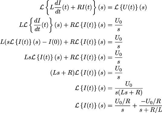
For the second line, I used the Laplace transform linearity, I took U0 / s from the table (usually, the Laplace transforms manually do not count, they use the tables).



To get the third line, use the derivative property.



The last line is obtained from the penultimate use of the method of indefinite decompositions . The meaning of this transition is to get a table function again. Of course, in the twenty-first century, it ’s useless .



Now it remains to apply the inverse Laplace transform (for the right side we look at the table) and we decided our diffur. The transition to the Laplace basis has turned the differential equation into the usual algebraic one!





Quick check of the result: after a few milliseconds, the inductance will no longer play a role, and we get the flowing current U_0 / R (Ohm's law). At the very beginning, the current flowing is zero and increases exponentially, and the rate of increase is directly dependent on the inductance. Sanity check passed.



The measurement file is here . Three columns, seconds, applied voltage (in volts), measured current (in amperes).



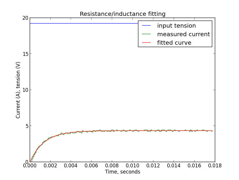
Here is the code that selects the resistance and inductance parameters for this experiment:





He says that the pair R = 4.4 Ohm, L = 6m Henry is well suited, here is the graph:

Input - sine

Repeat the procedure for a voltage sine wave with amplitude U0 and frequency F0. Apply the Laplace transform to equation (1), first to the right side:





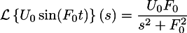
and then to the left:





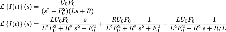
Now the inverse transformation will give us the following law of current flow:





Again, fast sanity check: zero current at the very beginning, a few milliseconds of transients (exponent, directly dependent on inductance). After some time, the current flowing is the weighted sum of the sine and cosine of the same frequency (the frequency is equal to the input, this is good). This amount gives a sinusoid slightly shifted in time. Great, the result is believable.



The measurements are here , and the parameter selection code is here . It gives approximately the same values ​​of resistance and inductance, which we needed. Here is the schedule:

Conclusion

Why not measure the parameters directly, why all this garden with microcontrollers? First, I have nothing to measure inductance. Yes, and measuring the resistance of the engine with an ohmmeter can have its own nuances.



Further, the parameters found at a high signal amplitude do not quite coincide with what is obtained at low voltages. It may be interesting (not considered here) to make a model not only of the engine, but of the whole system, including the non-linearity of the PWM driver.



Well, then it remains to develop a regulator that will take the required current strength at the input. Stay in touch!