Synthesis of images using deep neural networks. Lecture in Yandex
Suppose that this week in the Yandex blog on Habrahabr will be marked by neural networks. As we see, neural networks are now beginning to be used in very many areas, including search. It seems that it is “fashionable” to look for new areas of application for them, and in those areas where they have been working for some time, the processes are not so interesting.
However, events in the world of the synthesis of visual images prove the opposite. Yes, companies started using neural networks for image operations a few years ago - but this was not the end of the journey, but its beginning. Recently, the head of the Skoltech computer vision team and a big friend of Yandex and ShAD, Viktor Lempitsky, spoke about several new ways of applying networks to images. Since today's lecture is about pictures, it is very visual.
Under the cut - the decoding and most of the slides.
')
Good evening. Today I will talk about convolutional neural networks and I will assume that most of you have spent the last four years not on an uninhabited island, therefore, we heard something about convolutional deep neural networks and know approximately how they process data.
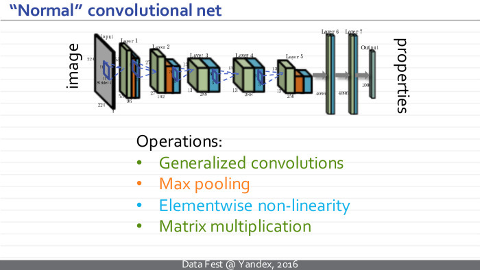
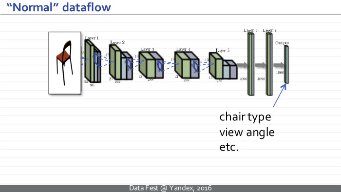
Therefore, I will spend the first two slides to tell exactly how they are applied to the images. They represent some architectures — complex functions with a large number of adjustable parameters, where elementary operations are of certain types, such as generalized convolutions, image size reduction, so-called pooling, element-wise nonlinearity applied to individual measurements, and multiplication by a matrix. Such a convolutional neural network takes a sequence of these operations, takes some image, for example, this cat.
Then it transforms a similar set of three images into a set of one hundred images, where each rectangle represents a really significant image specified in the MATLAB format.
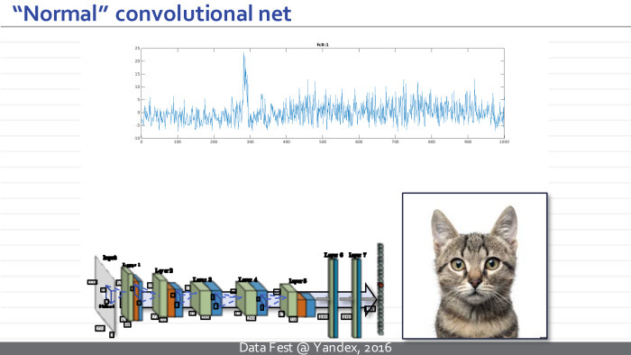
Next, some non-linearities are applied, and a new set of images is considered using the operations of generalized convolution. Several iterations occur, and at some point such a set of images is transformed into a multidimensional vector. After another series of multiplications on the matrix and elementwise non-linearities, this vector turns into a vector of properties of the input image, which we wanted to get to when we trained the neural network. For example, this vector can correspond to normalized probabilities or unnormalized values, where large values indicate that a particular class of objects is present in the image. In this example, the hump at the top corresponds to different breeds of cats, and the neural network thinks that this image contains a cat of one breed or another.
Neural networks that take pictures, process them in this order and get similar intermediate representations, I will call normal, ordinary or traditional convolutional networks.
But today I’ll speak mostly not about them, but about the new popular class of models, which I will call inverted or unfolded neural networks.
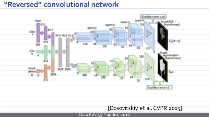
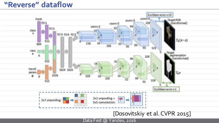
Here is an example of such an inverted neural network. This is a well-known model of the Freiburg group, Dosovitsky and colleagues, which is trained to take some vector of parameters and to synthesize an image that corresponds to them.
More specifically, the vector that encodes the class, a specific type of chair, and another vector that encodes the geometric parameters of the camera is fed to the input of this neural network. At the output, this neural network synthesizes an image of the chair and a mask separating the chair from the background.
As you can see, the difference between such a deployed neural network and the traditional one is that it does everything in the reverse order. Our image is no longer at the entrance, but at the exit. And the views that arise in this neural network are at first just vectors, and at some point turn into sets of images. Gradually, the images are combined with each other with the help of generalized convolutions, and the resulting images are obtained.
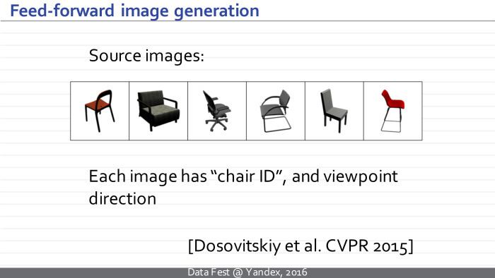
In principle, the neural network indicated on the previous slide was trained on the basis of synthetic images of chairs, which were obtained from several hundred CAD models of chairs. Each image is labeled with a chair class and camera parameters corresponding to the image.
An ordinary neural network will take a chair image at the entrance, predict the type of chair and the characteristics of the camera.
Dosovitsky's neural network does everything the other way around - it generates an image of the chair at the exit. I hope the difference is clear.
Interestingly, the components of an inverted neural network almost exactly repeat the components of a normal neural network. The only novelty and new module that arises is the module of reverse pooling, anpuling. This operation takes smaller pictures and converts them to larger pictures. This can be done in many ways that work about equally. For example, in their article they took small-sized maps, simply inserted zeros between them, then processed similar images.
This model turned out to be very popular, aroused a lot of interest and subsequent work. In particular, it turned out that such a neural network works very well, despite the seeming unusualness, exoticism and unnaturalness of such an idea - to deploy the neural network upside down, from left to right. It is capable not only of learning the learning set, but also of very good generalizations.
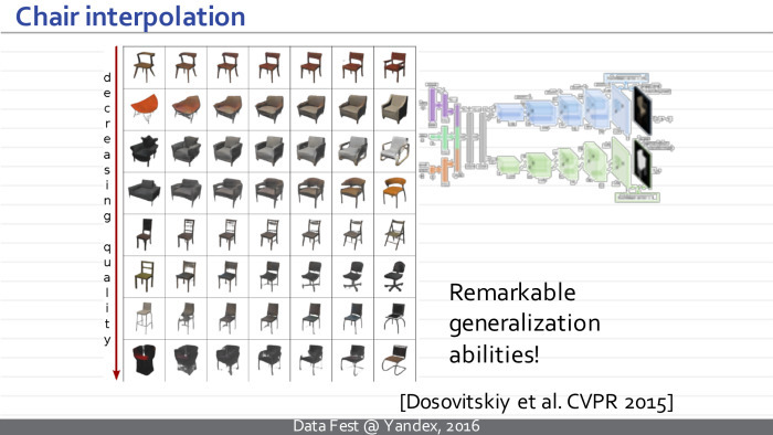
They showed that such a neural network can interpolate between two models of chairs and get a model as a mixture of chairs that were in the training set that the neural network had never seen. And the fact that these mixtures look like chairs, and not as arbitrary mixtures of pixels, says that our neural network is very well generalized.
If you ask yourself why this works so well, there are several answers. Two most convince me. First, why should it work badly if direct neural networks work well? Both direct and expanded networks use the same property of natural images that their statistics are local and the appearance of image slices does not depend on which part of the global image we are looking at. This property allows us to separate, reuse the parameters inside the convolutional layers of ordinary convolutional neural networks, and this property is used by the expanded networks, they are used successfully - it allows them to process and learn large amounts of data with a relatively small number of parameters.
The second property is less obvious and absent in direct neural networks: when we train a deployed network, we have much more training data than it seems at first glance. Each picture contains hundreds of thousands of pixels, and each pixel, although it is not an independent example, imposes restrictions on network parameters in one way or another. As a consequence, such a developed neural network can be effectively trained in a variety of images, which will be less than would be necessary for a good training of a direct network of a similar architecture with the same number of parameters. Roughly speaking, we can train a good model for chairs using thousands or tens of thousands of images, but not a million.
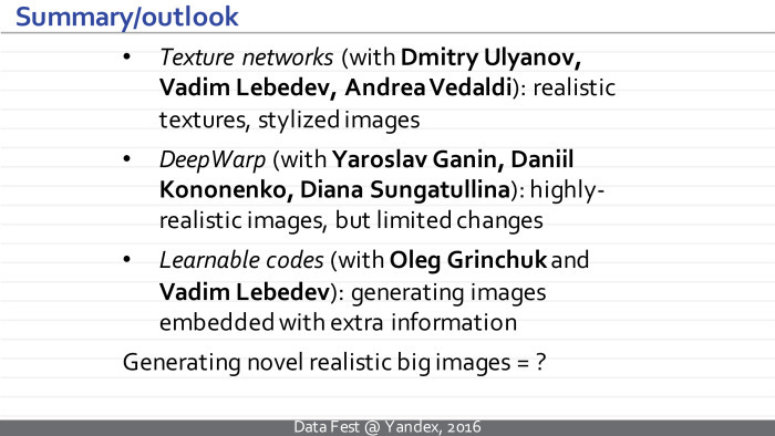
Today I would like to tell you about three ongoing projects related to deployed neural networks, or at least neural networks that produce an image at the output. I can hardly go into details - they are available on the links and in the articles of our group - but I hope such a run to the top will show you the flexibility and interestingness of this class of tasks. Maybe it will lead to some ideas about how neural networks can still be used to synthesize images.
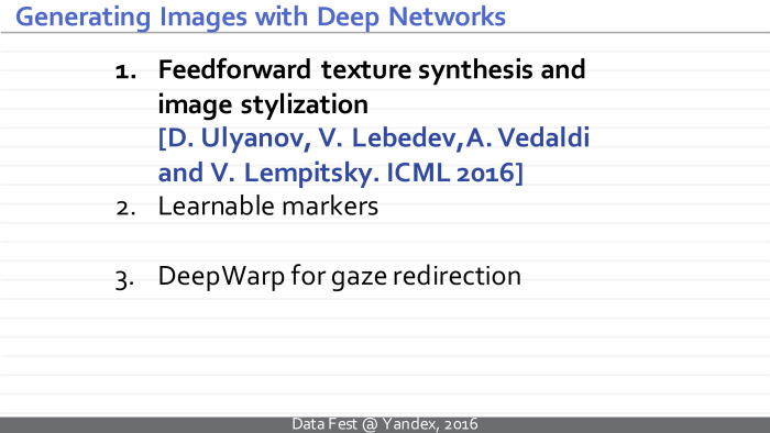
The first idea is devoted to the synthesis of textures and image styling. I will talk about the class of methods that matches what happens in Prisma and similar applications. All this developed in parallel and even slightly ahead of Prisma and similar applications. These methods are used in it or not - we probably don’t know, but we have some assumptions.
It all starts with the classic task of texture synthesis. People in computer graphics have been involved in this task for decades. Very briefly, it is formulated as follows: a texture sample is given and a method must be proposed that can generate new samples of the same texture for a given sample.
The task of texture synthesis in many ways rests on the task of comparing textures. How to understand that these two images correspond to similar textures, and these two - dissimilar? It is quite obvious that some simple approaches - for example, to compare three images pixel-by-pixel in pairs or to look at histograms - will not lead us to success, because the similarity of this pair will be the same as this one. Many researchers puzzled over how to define texture similarity measures, how to define some kind of texture handle, so that some simple measure in such advanced descriptors would say well whether textures are similar or not.
A year and a half ago, the group in Tübingen achieved a breakthrough. In fact, they generalized an earlier method based on wavelet statistics, which they replaced with activation statistics. It creates images and calls in some deep pre-ordinary network.
In their usual experiments, they took a large deep neural network trained for classification. Later it turned out that options are possible here: the network can even be deep with random weights, if they were initialized in a certain way.
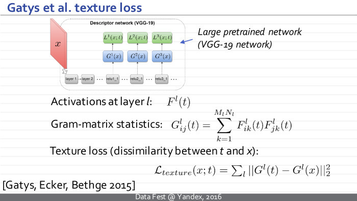
One way or another, statistics is defined as follows. Take an image, skip it through the first few convolutional layers of the neural network. On this layer we get a set of maps, images F l (t). t is a texture pattern. His set of image maps is on the l-layer.
Next, we consider texture statistics - it should somehow exclude from itself the parameters associated with the spatial location of an element. The natural approach is to take all pairs of cards in this view. We take all pairs of cards, count all pairwise scalar products between these pairs, take the i-th card and j-th card, then the k-th index goes through all possible spatial positions, we consider a similar scalar product and get the i, j coefficient, member Gram matrices. The Gram l-matrix, calculated in this way, describes our texture.
Further, when it is necessary to compare whether the two images are similar as textures, we simply take a certain set of layers: it can be one layer - then this amount includes one member. Or we can take several convolutional layers. Compare the Gram matrix, calculated in this way for these two images. We can compare them simply element by element.
It turns out that such statistics speaks very well about whether the two textures are similar or not - better than anything that was suggested before working on the slide.
Now that we have a very good measure that allows us to compare textures, we can take some random approximation, random noise. Let the current image be denoted as x and be some sample t. we will pass our current state through the neural network, look at its current Gram matrix. Next, using the back-propagation algorithm, we understand how to change the current propagation so that its Gram matrices inside the neural network become a bit more similar to the Gram matrices of the sample that we want to synthesize. Gradually, our noisy image will turn into a set of stones.

It works very well. Here is an example from their article. On the right is an example that we want to repeat, and on the left is a synthesized texture. The main problem is the time of work. For small images, it takes a lot of seconds.
The idea of this approach is to radically speed up the process of generating textures through the use of an inverted neural network.
It was proposed to train a new deployed neural network for this texture sample, which would accept some noise at the input and produce new texture samples.
Thus, x — which in the previous approach was some independent variable and we manipulated it, trying to create textures — now becomes a dependent variable, the output of a new neural network. It has its own parameters θ. The idea is to transfer training to a separate stage. Now we take and teach the neural network, adjusting its parameters so that for arbitrary noise vectors the resulting images have Gram matrices corresponding to our sample.
The loss functions remain the same, but now we have an additional module that we can pre-train in advance. The downside is that there is now a long-term learning stage, but the plus is as follows: after learning, we can synthesize new texture samples simply by synthesizing a new noise vector, passing it through a neural network, and it takes several tens of milliseconds.
Neural network optimization is also performed using the method of stochastic gradient descent, and our training is as follows: we synthesize the noise vector, pass it through the neural network, consider the Gram matrices, look at discrepancies, and back propagate through this entire path, we understand how to change the parameters of the neural network.
Here are some details of the architecture, I'll skip them. The architecture is fully convolutional, there are no fully connected layers, and the number of parameters is small. Such a scheme, in particular, does not allow the network to simply memorize the texture example provided to it so that it is issued again and again.
An example of the work of architecture. On the left is a specified pattern, and on the right are three examples that each of the three neural networks in the upper, lower and middle row provides for these samples. And this happens in a few tens of milliseconds, and not in seconds, as before. The architecture feature allows us to synthesize textures of arbitrary size.
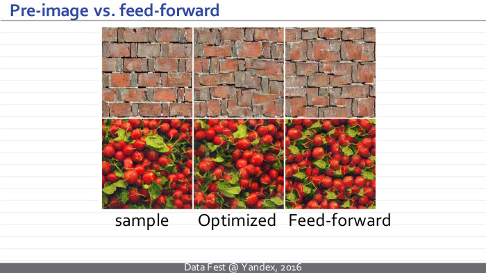
We can compare the result of the initial approach, which required optimization, and the new approach. We see that the quality of the resulting textures is comparable.
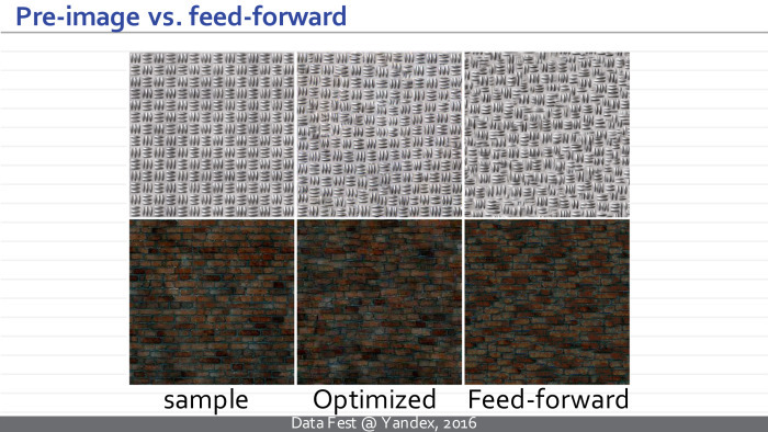
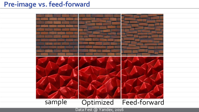
In the middle there is a sample of the texture obtained using the Gotiss method (inaudible - Ed.), Optimization, and on the right are examples of the textures produced by the neural network simply by converting the noise vector.
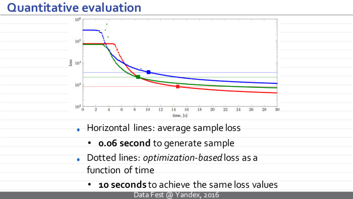
In fact, what happens can be interpreted as follows: the resulting neural network is a pseudo-optimizer and for some noise vectors it generates some good solution, which can then be improved, for example, by using an optimization approach. But usually this is not required, because the resulting solution visually has a slightly greater loss function, but in visual quality it is not much inferior or superior to what can be obtained by continuing optimization.
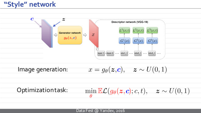
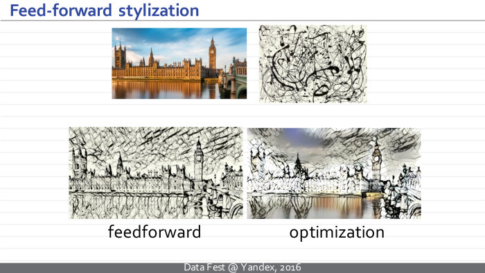
Interestingly, this approach can be summarized for image styling. We are talking about the processes when for a given photo and a given pattern of visual style, a new image is built that has the same content as the photo and the same visual style as the style sample.
The only change: our neural network will accept not only the noise vector, but also the image that needs to be stylized as input. She is trained for an arbitrary example of style.
The original article failed to build an architecture that would give results comparable in quality to the optimization approach. Later, Dmitry Ulyanov, the first author of the article, found an architecture that allowed him to radically improve the quality and achieve a quality of styling comparable to the optimization approach.
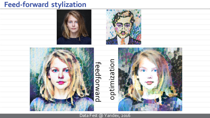
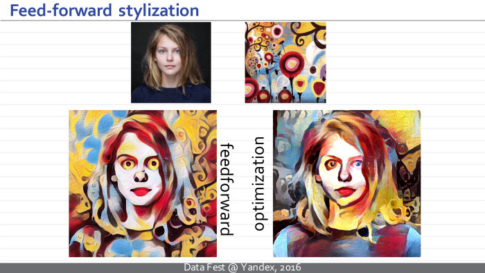
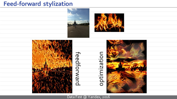
Here at the top is a photo and an example of the visual style, and below is the result of styling such a neural network, requiring several tens of milliseconds, and the result of the optimization method — which, in turn, requires multi-second optimization.
It is possible to discuss both quality and which stylization is more successful. But, I think, in this case, this is already an unclear question. In this example, I personally prefer the left version. Perhaps I am biased.
Here, probably, rather right.
But in this embodiment, the result is quite unexpected for me. It seems that the approach based on an inverted deployed neural network achieves better styling, while the optimization method is stuck somewhere in a poor local minimum or somewhere on a plateau — that is, it cannot fully stylize a photo.
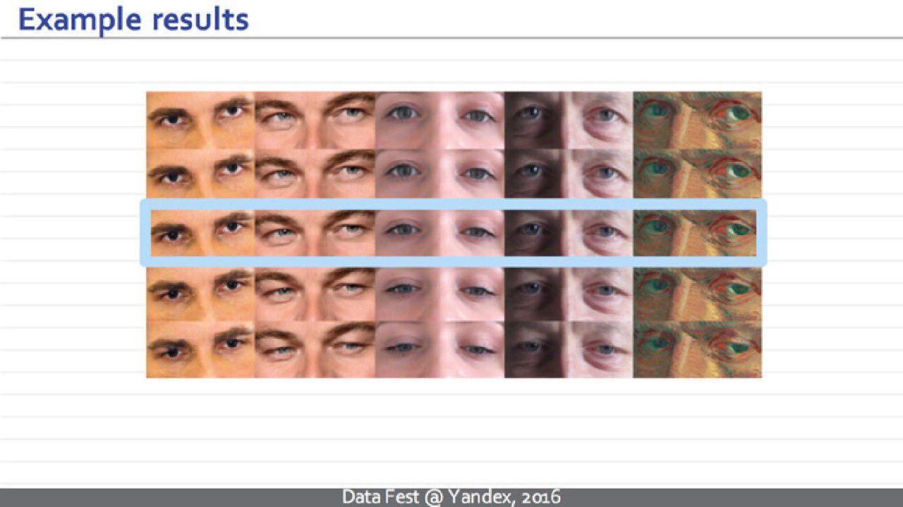
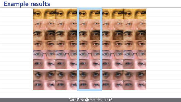
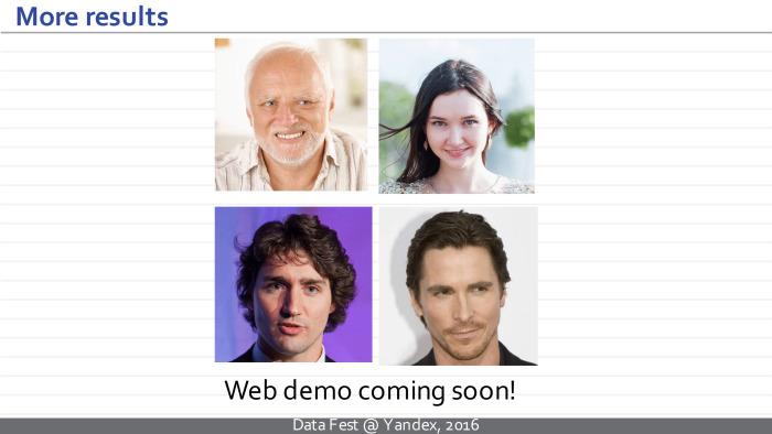
We’ll go back to styling. The second project is connected with the neural network, which solves the following problem. We wanted to build a network that could take a photo of a person’s face and redirect his view of this photo.

Why did we need to solve such an exotic problem? It turns out that there are at least two applications where it is relevant. The main thing for us - the task of improving eye contact with video conferencing. Probably, many people noticed that when you are talking on Skype or another video conferencing service, you cannot look at each other with the interlocutor, because the camera and the interlocutor's face are spaced apart by location.
Another application is the post-processing of movies. You have some kind of superstar whose minute of shooting is worth a million dollars. You shot a double, but this superstar looked the wrong way. And now it is necessary either to re-take the double, or to edit the direction of the look.
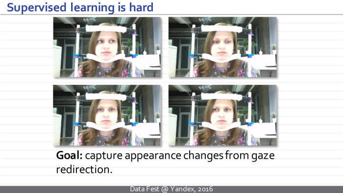
To solve this problem, we have collected a large number of sequences. Within them, we recorded the position of the head, the lighting - everything except the direction of the look. The protocol was such that we could track where the person was looking. Each frame is announced by the corresponding direction of view.
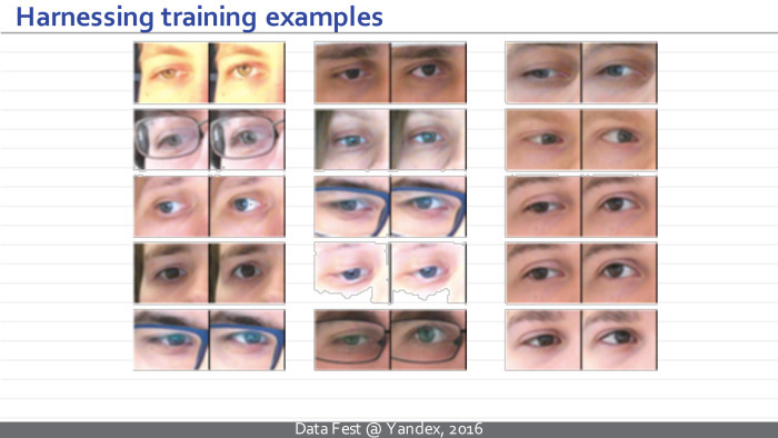
This allowed us to extract from this set of data a couple of examples for which we know: the only difference between the left and right images is the direction of gaze. For example, here in each case the difference is 15 degrees in the vertical direction.
We have practically moved from such a complex task to the classical problem of teaching with a teacher. We have an example on the left, and we need to generate an example on the right. Unfortunately, simply solving this problem with the help of a black box, as Sergey said, does not work. , - . , , . . , — , .
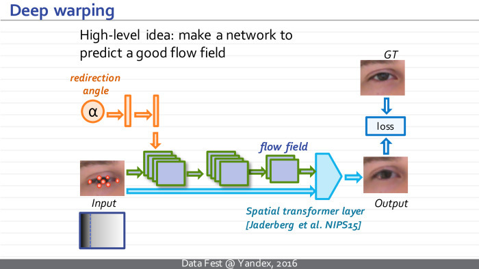
, , . , . . , , , . spatial transformer layer. , , torch .
, . , , , , , GT.
. , — , — , . , — , . , , .
. , , . , , , .
. - 15 . .
.
. , -, .
, . , . , .
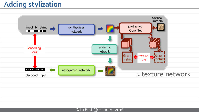
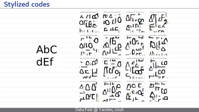
. , — — . . , , . , QR-, -.
, . - , , , .
— .
. . , , , , . , , .
, . , - . — , , . .
. , .
— . . , , .
, . , , — .
. , , , . , , , , - .
, — - , .
. , .
, , .
, , — .
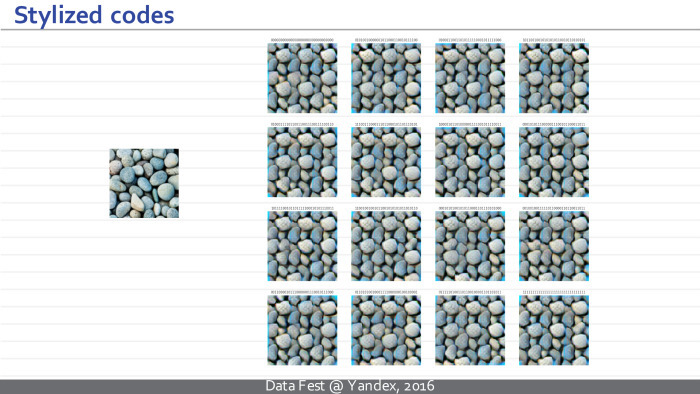
, , . , — . : , , , . , QR-, , , . — .
. .
. , , QR-, , - .
. . , . , , — , . , , . . Thank.
However, events in the world of the synthesis of visual images prove the opposite. Yes, companies started using neural networks for image operations a few years ago - but this was not the end of the journey, but its beginning. Recently, the head of the Skoltech computer vision team and a big friend of Yandex and ShAD, Viktor Lempitsky, spoke about several new ways of applying networks to images. Since today's lecture is about pictures, it is very visual.
Under the cut - the decoding and most of the slides.
')
Good evening. Today I will talk about convolutional neural networks and I will assume that most of you have spent the last four years not on an uninhabited island, therefore, we heard something about convolutional deep neural networks and know approximately how they process data.
Therefore, I will spend the first two slides to tell exactly how they are applied to the images. They represent some architectures — complex functions with a large number of adjustable parameters, where elementary operations are of certain types, such as generalized convolutions, image size reduction, so-called pooling, element-wise nonlinearity applied to individual measurements, and multiplication by a matrix. Such a convolutional neural network takes a sequence of these operations, takes some image, for example, this cat.
Then it transforms a similar set of three images into a set of one hundred images, where each rectangle represents a really significant image specified in the MATLAB format.
Next, some non-linearities are applied, and a new set of images is considered using the operations of generalized convolution. Several iterations occur, and at some point such a set of images is transformed into a multidimensional vector. After another series of multiplications on the matrix and elementwise non-linearities, this vector turns into a vector of properties of the input image, which we wanted to get to when we trained the neural network. For example, this vector can correspond to normalized probabilities or unnormalized values, where large values indicate that a particular class of objects is present in the image. In this example, the hump at the top corresponds to different breeds of cats, and the neural network thinks that this image contains a cat of one breed or another.
Neural networks that take pictures, process them in this order and get similar intermediate representations, I will call normal, ordinary or traditional convolutional networks.
But today I’ll speak mostly not about them, but about the new popular class of models, which I will call inverted or unfolded neural networks.
Here is an example of such an inverted neural network. This is a well-known model of the Freiburg group, Dosovitsky and colleagues, which is trained to take some vector of parameters and to synthesize an image that corresponds to them.
More specifically, the vector that encodes the class, a specific type of chair, and another vector that encodes the geometric parameters of the camera is fed to the input of this neural network. At the output, this neural network synthesizes an image of the chair and a mask separating the chair from the background.
As you can see, the difference between such a deployed neural network and the traditional one is that it does everything in the reverse order. Our image is no longer at the entrance, but at the exit. And the views that arise in this neural network are at first just vectors, and at some point turn into sets of images. Gradually, the images are combined with each other with the help of generalized convolutions, and the resulting images are obtained.
In principle, the neural network indicated on the previous slide was trained on the basis of synthetic images of chairs, which were obtained from several hundred CAD models of chairs. Each image is labeled with a chair class and camera parameters corresponding to the image.
An ordinary neural network will take a chair image at the entrance, predict the type of chair and the characteristics of the camera.
Dosovitsky's neural network does everything the other way around - it generates an image of the chair at the exit. I hope the difference is clear.
Interestingly, the components of an inverted neural network almost exactly repeat the components of a normal neural network. The only novelty and new module that arises is the module of reverse pooling, anpuling. This operation takes smaller pictures and converts them to larger pictures. This can be done in many ways that work about equally. For example, in their article they took small-sized maps, simply inserted zeros between them, then processed similar images.
This model turned out to be very popular, aroused a lot of interest and subsequent work. In particular, it turned out that such a neural network works very well, despite the seeming unusualness, exoticism and unnaturalness of such an idea - to deploy the neural network upside down, from left to right. It is capable not only of learning the learning set, but also of very good generalizations.
They showed that such a neural network can interpolate between two models of chairs and get a model as a mixture of chairs that were in the training set that the neural network had never seen. And the fact that these mixtures look like chairs, and not as arbitrary mixtures of pixels, says that our neural network is very well generalized.
If you ask yourself why this works so well, there are several answers. Two most convince me. First, why should it work badly if direct neural networks work well? Both direct and expanded networks use the same property of natural images that their statistics are local and the appearance of image slices does not depend on which part of the global image we are looking at. This property allows us to separate, reuse the parameters inside the convolutional layers of ordinary convolutional neural networks, and this property is used by the expanded networks, they are used successfully - it allows them to process and learn large amounts of data with a relatively small number of parameters.
The second property is less obvious and absent in direct neural networks: when we train a deployed network, we have much more training data than it seems at first glance. Each picture contains hundreds of thousands of pixels, and each pixel, although it is not an independent example, imposes restrictions on network parameters in one way or another. As a consequence, such a developed neural network can be effectively trained in a variety of images, which will be less than would be necessary for a good training of a direct network of a similar architecture with the same number of parameters. Roughly speaking, we can train a good model for chairs using thousands or tens of thousands of images, but not a million.
Today I would like to tell you about three ongoing projects related to deployed neural networks, or at least neural networks that produce an image at the output. I can hardly go into details - they are available on the links and in the articles of our group - but I hope such a run to the top will show you the flexibility and interestingness of this class of tasks. Maybe it will lead to some ideas about how neural networks can still be used to synthesize images.
The first idea is devoted to the synthesis of textures and image styling. I will talk about the class of methods that matches what happens in Prisma and similar applications. All this developed in parallel and even slightly ahead of Prisma and similar applications. These methods are used in it or not - we probably don’t know, but we have some assumptions.
It all starts with the classic task of texture synthesis. People in computer graphics have been involved in this task for decades. Very briefly, it is formulated as follows: a texture sample is given and a method must be proposed that can generate new samples of the same texture for a given sample.
The task of texture synthesis in many ways rests on the task of comparing textures. How to understand that these two images correspond to similar textures, and these two - dissimilar? It is quite obvious that some simple approaches - for example, to compare three images pixel-by-pixel in pairs or to look at histograms - will not lead us to success, because the similarity of this pair will be the same as this one. Many researchers puzzled over how to define texture similarity measures, how to define some kind of texture handle, so that some simple measure in such advanced descriptors would say well whether textures are similar or not.
A year and a half ago, the group in Tübingen achieved a breakthrough. In fact, they generalized an earlier method based on wavelet statistics, which they replaced with activation statistics. It creates images and calls in some deep pre-ordinary network.
In their usual experiments, they took a large deep neural network trained for classification. Later it turned out that options are possible here: the network can even be deep with random weights, if they were initialized in a certain way.
One way or another, statistics is defined as follows. Take an image, skip it through the first few convolutional layers of the neural network. On this layer we get a set of maps, images F l (t). t is a texture pattern. His set of image maps is on the l-layer.
Next, we consider texture statistics - it should somehow exclude from itself the parameters associated with the spatial location of an element. The natural approach is to take all pairs of cards in this view. We take all pairs of cards, count all pairwise scalar products between these pairs, take the i-th card and j-th card, then the k-th index goes through all possible spatial positions, we consider a similar scalar product and get the i, j coefficient, member Gram matrices. The Gram l-matrix, calculated in this way, describes our texture.
Further, when it is necessary to compare whether the two images are similar as textures, we simply take a certain set of layers: it can be one layer - then this amount includes one member. Or we can take several convolutional layers. Compare the Gram matrix, calculated in this way for these two images. We can compare them simply element by element.
It turns out that such statistics speaks very well about whether the two textures are similar or not - better than anything that was suggested before working on the slide.
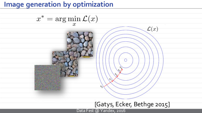
Now that we have a very good measure that allows us to compare textures, we can take some random approximation, random noise. Let the current image be denoted as x and be some sample t. we will pass our current state through the neural network, look at its current Gram matrix. Next, using the back-propagation algorithm, we understand how to change the current propagation so that its Gram matrices inside the neural network become a bit more similar to the Gram matrices of the sample that we want to synthesize. Gradually, our noisy image will turn into a set of stones.
It works very well. Here is an example from their article. On the right is an example that we want to repeat, and on the left is a synthesized texture. The main problem is the time of work. For small images, it takes a lot of seconds.
The idea of this approach is to radically speed up the process of generating textures through the use of an inverted neural network.
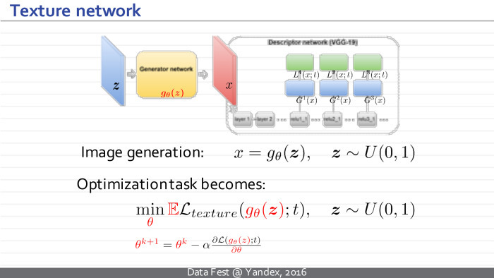
It was proposed to train a new deployed neural network for this texture sample, which would accept some noise at the input and produce new texture samples.
Thus, x — which in the previous approach was some independent variable and we manipulated it, trying to create textures — now becomes a dependent variable, the output of a new neural network. It has its own parameters θ. The idea is to transfer training to a separate stage. Now we take and teach the neural network, adjusting its parameters so that for arbitrary noise vectors the resulting images have Gram matrices corresponding to our sample.
The loss functions remain the same, but now we have an additional module that we can pre-train in advance. The downside is that there is now a long-term learning stage, but the plus is as follows: after learning, we can synthesize new texture samples simply by synthesizing a new noise vector, passing it through a neural network, and it takes several tens of milliseconds.
Neural network optimization is also performed using the method of stochastic gradient descent, and our training is as follows: we synthesize the noise vector, pass it through the neural network, consider the Gram matrices, look at discrepancies, and back propagate through this entire path, we understand how to change the parameters of the neural network.
Here are some details of the architecture, I'll skip them. The architecture is fully convolutional, there are no fully connected layers, and the number of parameters is small. Such a scheme, in particular, does not allow the network to simply memorize the texture example provided to it so that it is issued again and again.
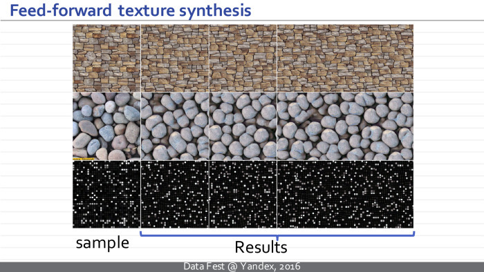
An example of the work of architecture. On the left is a specified pattern, and on the right are three examples that each of the three neural networks in the upper, lower and middle row provides for these samples. And this happens in a few tens of milliseconds, and not in seconds, as before. The architecture feature allows us to synthesize textures of arbitrary size.
We can compare the result of the initial approach, which required optimization, and the new approach. We see that the quality of the resulting textures is comparable.
In the middle there is a sample of the texture obtained using the Gotiss method (inaudible - Ed.), Optimization, and on the right are examples of the textures produced by the neural network simply by converting the noise vector.
In fact, what happens can be interpreted as follows: the resulting neural network is a pseudo-optimizer and for some noise vectors it generates some good solution, which can then be improved, for example, by using an optimization approach. But usually this is not required, because the resulting solution visually has a slightly greater loss function, but in visual quality it is not much inferior or superior to what can be obtained by continuing optimization.
Interestingly, this approach can be summarized for image styling. We are talking about the processes when for a given photo and a given pattern of visual style, a new image is built that has the same content as the photo and the same visual style as the style sample.
The only change: our neural network will accept not only the noise vector, but also the image that needs to be stylized as input. She is trained for an arbitrary example of style.
The original article failed to build an architecture that would give results comparable in quality to the optimization approach. Later, Dmitry Ulyanov, the first author of the article, found an architecture that allowed him to radically improve the quality and achieve a quality of styling comparable to the optimization approach.
Here at the top is a photo and an example of the visual style, and below is the result of styling such a neural network, requiring several tens of milliseconds, and the result of the optimization method — which, in turn, requires multi-second optimization.
It is possible to discuss both quality and which stylization is more successful. But, I think, in this case, this is already an unclear question. In this example, I personally prefer the left version. Perhaps I am biased.
Here, probably, rather right.
But in this embodiment, the result is quite unexpected for me. It seems that the approach based on an inverted deployed neural network achieves better styling, while the optimization method is stuck somewhere in a poor local minimum or somewhere on a plateau — that is, it cannot fully stylize a photo.
We’ll go back to styling. The second project is connected with the neural network, which solves the following problem. We wanted to build a network that could take a photo of a person’s face and redirect his view of this photo.
Why did we need to solve such an exotic problem? It turns out that there are at least two applications where it is relevant. The main thing for us - the task of improving eye contact with video conferencing. Probably, many people noticed that when you are talking on Skype or another video conferencing service, you cannot look at each other with the interlocutor, because the camera and the interlocutor's face are spaced apart by location.
Another application is the post-processing of movies. You have some kind of superstar whose minute of shooting is worth a million dollars. You shot a double, but this superstar looked the wrong way. And now it is necessary either to re-take the double, or to edit the direction of the look.
To solve this problem, we have collected a large number of sequences. Within them, we recorded the position of the head, the lighting - everything except the direction of the look. The protocol was such that we could track where the person was looking. Each frame is announced by the corresponding direction of view.
This allowed us to extract from this set of data a couple of examples for which we know: the only difference between the left and right images is the direction of gaze. For example, here in each case the difference is 15 degrees in the vertical direction.
We have practically moved from such a complex task to the classical problem of teaching with a teacher. We have an example on the left, and we need to generate an example on the right. Unfortunately, simply solving this problem with the help of a black box, as Sergey said, does not work. , - . , , . . , — , .
, , . , . . , , , . spatial transformer layer. , , torch .
, . , , , , , GT.
. , — , — , . , — , . , , .
. , , . , , , .
. - 15 . .
.
. , -, .
, . , . , .
. , — — . . , , . , QR-, -.
, . - , , , .
— .
. . , , , , . , , .
, . , - . — , , . .
. , .
— . . , , .
, . , , — .
. , , , . , , , , - .
, — - , .
. , .
, , .
, , — .
, , . , — . : , , , . , QR-, , , . — .
. .
. , , QR-, , - .
. . , . , , — , . , , . . Thank.
Source: https://habr.com/ru/post/314508/
All Articles