Using FPGA to calculate microtubule depolymerization using Brownian dynamics
Everything is ready to tell Habr to the audience about the application of FPGA in the field of scientific high-performance computing. And how on this task it was necessary to significantly jump off the GPU (Nvidia K40) not only in the performance metric per watt, but simply in terms of computation speed. As an FPGA platform, a Xilinx Virtex-7 2000t crystal connected via a PCIe to a host computer was used. To create a hardware computational core, C ++ (Vivado HLS) was used.
Under the cut the text of our original article. There, as usually happens, at first there is a long description of why this is all necessary and the model, if you don’t want to read it, you can go straight to the implementation, and then look at the model if necessary. On the other hand, without at least a quick acquaintance with the model, the reader will not be able to get the impression of which complex calculations can be implemented on FPGA.
annotation
In this paper, we consider the hardware implementation of the calculation of protein microtubule depolymerization using the method of Brownian dynamics on a Xilinx Virtex-7 programmable logic integrated circuit (FPGA) chip using a high-level translator from the C language Vivado HLS. The implementation on the FPGA is compared with parallel implementations of the same algorithm on the multi-core Intel Xeon processor and the Nvidia K40 graphics processor according to the criteria of performance and energy efficiency. The algorithm works on Brownian times and therefore requires a large number of normally distributed random numbers. The original serial code was optimized for the multicore architecture using OpenMP, for the graphics processor using OpenCL, and the implementation on the FPGA was obtained using the high-level translator Vivado HLS. The paper shows that implementation on FPGA is 17 times faster than CPU and 11 times faster than GPU. As for energy efficiency (performance per watt), the FPGA was 160 times better than the CPU and 80 times better than the GPU. The FPGA-accelerated application was developed using an SDK that includes a ready-made FPGA project, having a PCI Express interface for communicating with a host computer, and software libraries for communicating a host application with an FPGA accelerator. From the end developer, it was only necessary to develop the computational core of the C-language algorithm in the Vivado HLS environment, and did not require special FPGA development skills.
Introduction
High-performance computing is carried out on processors (CPUs), clustered and / or having hardware accelerators — graphics processors on video cards (GPUs) or programmable logic integrated circuits (FPGAs) [1]. The modern processor itself is an excellent platform for high-performance computing. The advantages of the CPU include a multi-core architecture with a common coherent cache, support for vector instructions, high frequency, as well as a huge set of software tools, compilers and libraries, providing high programming flexibility. The high performance of the GPU platform is based on the ability to run thousands of parallel computing threads on independent hardware cores. Well-known development tools (CUDA, OpenCL) are available for the GPU, reducing the threshold for using the GPU platform for applied computing tasks. Despite this, in recent years, FPGAs have increasingly been used as a platform for speeding up tasks, including those using real computation [2]. FPGAs have a unique property that distinguishes them sharply from the CPU and GPU, namely the ability to build a pipeline hardware circuit for a specific computational algorithm. Therefore, despite the significantly lower clock frequency at which FPGAs operate (compared to CPU and GPU), some algorithms on FPGA achieve greater performance [3] - [5]. On the other hand, a lower operating frequency means less power consumption, and FPGA is almost always more efficient than a CPU and a GPU, if you use the performance per watt metric [5].
One of the classic applications requiring high-performance computing is the molecular dynamics method used to calculate the motion of systems of atoms or molecules. Within this method, interactions between atoms and molecules are described within the laws of Newtonian mechanics using interaction potentials. The calculation of the interaction forces is carried out iteratively and represents a significant computational complexity, given the large number of atoms / molecules in the system and a large number of calculated iterations. Acceleration of molecular dynamics calculations has received much attention in the literature in various systems: supercomputers [6], clusters [7], machines specialized in molecular dynamics calculations [8] - [10], machines with GPU-based accelerators [11] and FPGA [12] - [17]. It has been demonstrated that FPGA can be a competitive alternative as a hardware accelerator for molecular dynamic computing in many cases, but today there is no consensus on which tasks and algorithms it is more profitable to use the FPGA platform. In this paper, we consider an important particular case of molecular dynamics — the Brownian dynamics. The main feature of the Brownian dynamics method in comparison with molecular dynamics is that the molecular system is modeled more roughly, i.e. The elementary objects of modeling are not individual atoms, but larger particles, such as individual macromolecule domains or whole macromolecules. Solvent molecules and other small molecules are not explicitly modeled, and their effects are accounted for as random force. Thus, it is possible to significantly reduce the dimension of the system, which allows us to increase the time interval covered by model calculations by orders of magnitude. We are not aware of the attempts in the literature to investigate the effectiveness of FPGA in comparison with alternative platforms for accelerating Brownian dynamics problems. Therefore, we have undertaken a study of this issue on the example of the problem of simulating the microtubule depolymerization using the method of Brownian dynamics. Microtubules are tubes with a diameter of about 25 nm and a length of from several tens of nanometers to tens of microns, consisting of tubulin protein and forming part of the inner skeleton of living cells. A key feature of microtubules is their dynamic instability, i.e. the ability to spontaneously switch between the phases of polymerization and depolymerization [18]. This behavior is primarily important for the capture and movement of chromosomes by microtubules during cell division. In addition, microtubules play an important role in intracellular transport, the movement of cilia and flagella, and the maintenance of cell shape [19].
The mechanisms underlying microtubule operation have been explored for several decades, but only recently the development of computational technologies has made it possible to describe the behavior of microtubules at the molecular level. The most detailed molecular model of the microtubule dynamics, recently created by our group based on the Brownian dynamics method, was implemented on the basis of the CPU and made it possible to calculate the polymerization / depolymerization times of microtubules on the order of a few seconds [20]. This shed light on a number of important aspects of the dynamics of microtubules, however, nevertheless, many key experimentally observed phenomena remained outside the framework of a theoretical description, since they occur in microtubules at times of tens and even hundreds of seconds [21]. Thus, for a direct comparison of theory and experiment, it is critical to achieve acceleration of calculations of the dynamics of microtubules by at least an order of magnitude.
In this paper, we explore the possibility of accelerating the calculations of Brownian microtubule dynamics on FPGA and compare the results obtained with the implementation of the same microtubule dynamics algorithm on three different platforms, according to the criteria of performance and energy efficiency.
Mathematical model
General information about the structure of microtubules
Structurally, a microtubule is a cylinder consisting of 13 chains - protofilaments.

The figure on the left shows the microtubule model diagram. The subunits of tubulin are shown in gray, the centers of interaction between them are shown in black dots. On the right is a view of the energy potentials of interaction between tubulins.
Each protofilament is constructed from tubulin protein dimers. Neighboring protofilaments are connected to each other by lateral bonds and are shifted relative to each other by a distance of 3/13 of the length of one monomer, so that the microtubule has helicity. During polymerization, tubulin dimers are attached to the ends of protofilaments, and microtubule protofilaments tend to adopt a direct conformation. During depolymerization, the lateral bonds between the protofilaments at the end of the microtubule are broken, and the protofilaments twist out. At the same time, tubulin oligomers are randomly detached from them.
Simulation of microtubule depolymerization by the method of Brownian dynamics
The molecular model of the microtubule used here was first presented in [20]. Since the objective of this study was to compare the performance of various computing platforms, we limited ourselves to modeling only the depolymerization of a microtubule.
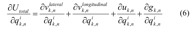
In short, a microtubule was modeled as a set of spherical particles representing tubulin monomers. Monomers could move only in the corresponding radial plane, i.e. in the plane passing through the microtubule axis and the corresponding protofilament. Thus, the position and orientation of each monomer was completely determined by three coordinates: two Cartesian coordinates of the center of the monomer and an orientation angle. Each monomer had four interaction centers on its surface: two side interaction centers and two longitudinal interaction centers. The energy of the tubulin-tubulin interaction depended on the distance r between the interaction sites on the surface of the adjacent subunits and on the angle of inclination between the neighboring tubulin monomers in the protofilament. Lateral and longitudinal interactions between tubulin dimers were determined by the potential, which has the following form:
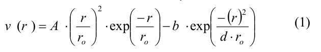
where A and b determine the depth of the potential well and the height of the energy barrier, r0 and d are the parameters defining the width of the potential well and the shape of the potential as a whole. Parameter A assumed different values for side and longitudinal links, so that side interactions were weaker than longitudinal, all other parameters were the same for both types of links (the full list of parameters and their values is presented in Table 1 in [20]). Longitudinal interactions inside the dimer were modeled as inseparable springs with a quadratic energy potential u_r:
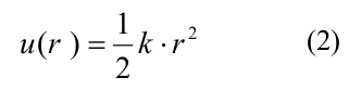
where k is the stiffness of the tubulin-tubulin interaction. The bending energy g (χ) is associated with the rotation of the monomers relative to each other and was also described by a quadratic inseparable function:

where χ is the angle between adjacent tubulin monomers in the protofilament, χ 0 is the equilibrium angle between the two monomers, B is the bending stiffness. The total energy of the microtubule was recorded as follows:
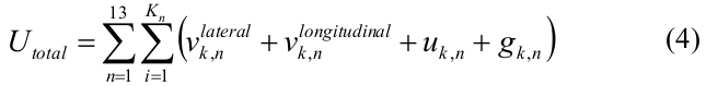
where n is the protofilament number, i is the monomer number in the nth protofilament, Kn is the number of tubulin subunits in the nth protofilament;
The evolution of the system was calculated using the method of Brownian dynamics [22]. The initial microtubule configuration was a short “seed” containing 12 tubulin monomers in each protofilament. We considered only MT depolymerization and modeled all tubulins with the equilibrium angle χ 0 = 0.2 rad. The coordinates of all the monomers of the system at the i-th iteration were expressed as follows:
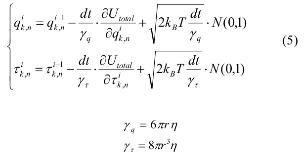
where dt is the time step, U total is expressed in terms of (4), k_B is the Boltzmann constant, T is the temperature, N (0.1) is a random number from the normal distribution, generated using the Mersenne vortex algorithm [23]. γ q and γ τ are viscous drag coefficients for shear and rotation, respectively, calculated for spheres of radius r = 2 nm.
The total energy derivative with respect to the independent coordinates q {k, n} was expressed through the lateral, longitudinal components of the interaction energy between neighboring dimers and within the dimer, as well as the bending energy:
To speed up the calculations, analytical expressions for
all energy gradients:
It should be noted that the size of this task is relatively small. We considered only 12 layers of monomers, which gives a total number of particles equal to 156. However, this does not diminish the significance of the calculations, since in real calculations, it is sufficient to calculate the position of the last several (about 10) words of monomers, since with the growth of microtubules, the tubulin molecules furthest from the end of the microtubule form a stable cylindrical configuration, and there is no point in taking them into account.
Pseudocode calculation algorithm
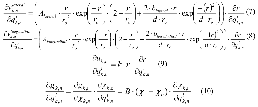
The algorithm is iterative in time with a step of 0.2 ns. There are an array of three-dimensional coordinates of molecules, as well as arrays of transverse (lateral) and longitudinal (longitudinal) forces. At each iteration in time, two nested cycles with molecules are performed sequentially, in the first one, the interaction forces are calculated from known coordinates, in the second, the coordinates themselves are updated. In the cycle of calculating the interaction forces, it is necessary to read the coordinates of three molecules, one central and two adjacent (“left” and “top”, see Fig.2), and the result of the calculation will be the transverse interaction between the central and left molecules and the force of the longitudinal interaction between the central and top.
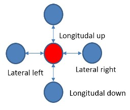
Fig. 2. Layout of interacting subunits in the microtubule model
As a result, after this cycle, all the interaction forces between all molecules are calculated. In the cycle of updating the coordinates by known forces, the changes of coordinates are calculated, and random additives are also taken into account to account for Brownian motion. Thus, the pseudo-code of the algorithm can be written as follows.
: M = {x, y, teta}. . : M K for t in {0.. K-1} do for i in {0.. 13} // for j in {0.. 12} do // Mc <- M[i,j] Ml <- M[i+1,j] Mu <- M[i,j+1] // (7, 8, 9, 10) F_lat[i,j] <- calc_calteral(Mc, Ml) F_long[i,j] <- calc_long(Mc, Mu) end for end for for i in {0.. 13} for j in {0.. 12} do // (5) M[i,j] <- update_coords(F_lat[i,j], F_long[i,j]) end for end for end for Software implementation on CPU and GPU
CPU implementation
An attempt was made to maximally parallelize code on an Intel Xeon E5-2660 2.20GHz CPU running on Ubuntu 12.04 OS using the OpenMP library. The parallel section started before the time cycle. The cycles of calculating the interaction forces and coordinate updates were parallelized using the omp for schedule (static) directive, and barrier synchronization was inserted between the cycles. Arrays containing interaction forces and molecular coordinates were declared private for each flow.
When implementing the calculations on the CPU, it was found that the size of the task did not allow it to be parallelized effectively. The dependence of the execution time of one iteration on the number of parallel threads was non-monotonic. The minimum time for calculating one iteration over time was obtained using only 2 threads (CPU cores). This is explained by the fact that, with an increase in the number of threads, time increases for copying data between threads and for synchronizing them. At the same time, the size of the task is very small, so that the gain from the increase in the number of cores exceeds this overhead. At the same time, experiments have shown that the task scales poorly with increasing size (weak scaling), i.e. with a simultaneous increase in the size of the problem and the number of parallel threads, the computation time remained approximately the same. As a result, the best result on this CPU was 22 μs per iteration with the use of two CPU cores. The code was not vectorized due to the complexity of computing the interaction forces.
GPU implementation
We run an OpenCL implementation on an Nvidia Tesla K40 graph processor. The cycles that calculate the interaction forces and coordinate updates were parallelized, the main time loop was iterative. Two options were implemented - with one and several working groups (work groups). In the first case, one workflow was allocated (work item) for each molecule. In each flow there was a cycle in time in which the forces and coordinates of the flow molecule were calculated. At the same time, barrier synchronization was applied after the forces were calculated and after the coordinates were updated. In this case, the participation of the host was not required for computations; he was only involved in managing and launching the cores.
In the second case, there were two types of flows, in one, the forces for one molecule were simply calculated, in the second, the coordinates were updated. The main time loop was on the host, which controlled the launch and synchronization of the cores at each iteration of the time loop.
The highest performance was obtained in calculations with one group of flows and barrier synchronization between them. Without using pseudo-random number generators, one iteration was calculated for 5 μs, if one number generator was used for all streams, the operation time increased to 9 μs, and with maximum shared memory, 7 independent generators could be turned on, while one iteration in time was 14 µs, which was 1.57 times faster than the implementation on the CPU.
The load on the GPU cores was 7% of a single multiprocessor (SM), while the total memory, where the arrays of forces, coordinates, and data buffers of pseudo-random numbers were located, was 100% full. Those. on the one hand, the size of the task was obviously small to fully load the GPU, on the other hand, as the size of the task increased, we would have to use global DDR memory, which could limit the growth in performance.
FPGA implementation
Platform Description
Calculations on the FPGA were made on the platform of RB-8V7 manufactured by the company NPO Rost. It is a 1U rack unit. The block consists of 8 FPGA Xilinx Virtex-7 2000T crystals. Each FPGA has 1 GB of external DDR3 memory and a PCI Express x4 2.0 interface to an internal PCIe switch. The unit has two PCIe x4 3.0 interfaces to the host computer via optical cables that must be connected to a special adapter installed in the host computer.
As the host computer, a server with an Intel Xeon E5-2660 2.20 GHz CPU was used, running under Ubuntu 12.04 LTS OS - the same as for computing just on the CPU using OpenMP. Software running on the host computer's CPU “sees” the RB-8V7 as 8 independent FPGA devices connected via the PCI Express bus. Next, the interaction of the CPU with only one FPGA XC7V72000T will be described, while the system allows the use of FPGA independently and in parallel.
The FPGA accelerated application was developed using the SDK with the following model. The host program (hereinafter referred to as the CPU) runs the main program that uses the FPGA accelerator for the most computationally intensive procedures. The CPU transfers data to the accelerator and back through the external DDR memory connected to the FPGA, and also controls the operation of the computing core in the FPGA. The computational core is created in advance in C / C ++, verified and translated into RTL code using the Vivado HLS tool. The RTL code of the computational core is inserted into the main FPGA project, in which the necessary control and data transfer logic, including the PCI Express core, DDR controller and bus on chip, is already implemented (Fig. 3). The main FPGA project is sometimes called the Board Support Package (BSP), it is developed by the equipment manufacturer, and the user is not required to modify it. After launch, the HLS computational core itself turns into DDR memory, reads out the input data buffer for processing and writes the result of the calculations there. At the C ++ level, memory access occurs through the argument of the top-level function of the computational kernel of the pointer type.
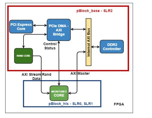
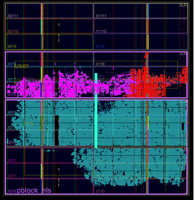
Fig. 3. Block diagram of the FPGA project. The blue and yellow colors indicate the blocks that are part of the BSP. Green indicates computational HLS cores. Also denoted is the breakdown of project kernels into blocks (pBlocks) for imposing space constraints during tracing.
To create an accelerated application, a methodology consisting of several steps was developed. First, the original sequential code was compiled in the Vivado HLS environment, and it was verified that the code compiled in this way does not change the output data of the reference serial code. Secondly, the main computational and suitable for acceleration part was separated from this code; this part was separated from the main code using the wrapper function. After that, two copies of such a function were created and the logic of checking that the results of both parts were consistent. The first copy was the reference implementation of the algorithm in Vivado HLS, and the second was optimized for translation into RTL code. Optimizations included code rewriting, such as using static arrays instead of dynamic ones, using special functions for input / output to the HLS core, methods of saving memory and re-using the results of calculations. After each change, the result of the function was compared with the result of the reference implementation. Another optimization method was the use of special Vivado HLS directives that do not change the logical behavior, but affect the final performance of the RTL code. At this stage, one should remain until satisfactory preliminary results of C-to-RTL translation are obtained, such as circuit performance and resources occupied.
The next stage is the implementation of the developed computational core in the Vivado system outside the context of the main project. Here the task is to achieve the absence of temporary errors of the already diluted design inside the developed computational core. If temporary errors are observed at this stage, then you can apply other implementation parameters, or return to the previous stage and try to change the C ++ code or use other directives.
At the next stage, it is necessary to implement the computational core together with the main project and its temporal and spatial constraints. At this stage it is also necessary to achieve the absence of temporary errors. If they are observed, then you can either change the frequency of the computational scheme, impose other spatial constraints on the placement of the scheme on the chip, or again
change C ++ code and / or use other directives.
The last stage of development is a test for compliance with the results obtained on a real run in hardware and with the help of a reference model on the CPU. It takes place over a short period of time, and it is considered that on longer launches (when it is already problematic to compare with the CPU) the FPGA solution gives the correct results.
Work in the environment Vivado HLS
We used two Vivado HLS cores (Fig. 3): the main core that implements the microtubule molecular dynamics algorithm (MT core), and the core for generating pseudo-random numbers (RAND core). We had to divide the algorithm into two computational cores for the following reason. The FPGA Virtex-7 2000T crystal is the largest FPGA crystal in the Virtex-7 family on the market. It actually consists of four silicon crystals, connected on a substrate by a multitude of compounds and integrated into a single chip package. In Xilinx terminology, each such crystal is called SLR (Super Logic Region). When using such large FPGAs, there are always problems with circuits crossing the SLR boundaries. Xilinx recommends inserting registers onto such circuits on both sides of the SLR boundary.
The full HLS core, including both the MT and RAND cores, required more hardware resources than was available in the same SLR, so there were chains that crossed the border of independent silicon crystals. At the stage of translation from C ++ language in RTL, Vivado HLS does not “know” anything about which chains will subsequently cross the border, and therefore cannot insert additional synchronization registers in advance. Therefore, we decided to divide the cores into two, spatially limit them to different SLRs and insert synchronization registers to the interface circuits between the cores at the RTL level.
MT kernel
This algorithm is very well suited for implementation on an FPGA; therefore, for a relatively small amount of data from memory (coordinates of two molecules), it is necessary to calculate a complex function of interaction forces and it is possible to build a long computing pipeline.
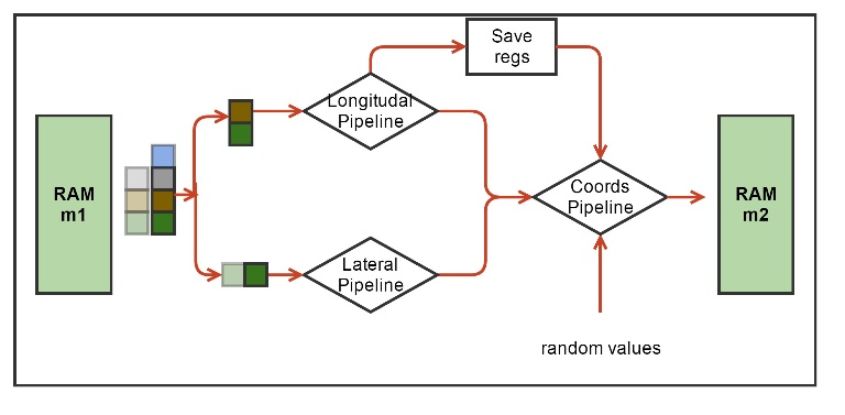
Fig. 4. The block diagram of the hardware computational procedure for the MT kernel. Green denotes hardware blocks of memory for storing the coordinates of molecules. Indicated are the computational force pipelines and coordinate updates, as well as the Save Regs block for storing intermediate results of calculations. Pseudo-random numbers enter the coordinate update pipeline from another HLS core.
Each molecule, i.e. tubulin monomer, interacts with only four of its neighbors (Fig. 2). At each iteration in time, you must first calculate the interaction force, and then update the coordinates of the molecules. The functions of calculating the interaction forces include a set of arithmetic, exponential and trigonometric operators. Our first task was to synthesize a pipeline for these functions. The working data type was float. Vivado HLS synthesized such functions as pipelines operating at 200 MHz, with a latency of about 130 cycles. At the same time, the conveyors were one-stroke (or, as they say, with an initialization interval equal to 1), which means that they could take the coordinates of new molecules at the input each stroke, and then after the initial delay (latency), give the updated values of the forces also each measure. Interaction output forces were used to update the coordinates, which was also pipelined. To update each coordinate of each molecule, we needed independent pseudo-random, normally distributed numbers derived from another HLS nucleus. If we take three molecules ("current", "left" and "top"), then it turned out possible to combine the conveyors for calculating forces and updating coordinates into one conveyor that implements all the calculations for one molecule. Such a conveyor had a latency of 191 cycles (Fig. 4).
The algorithm passes through all the molecules in the cycle. At each iteration of the cycle, it is necessary to have the coordinates of three molecules: one molecule is considered as “current”, there are also “left” and “right” molecules. The interaction forces between these three molecules are calculated accordingly. Then, when updating the coordinates of the current molecule, the left and upper components of the interaction forces were taken at the current iteration, and the lower and right components were taken either from boundary conditions or from previous iterations from the Save Regs local register file (Fig. 4).
The number of N molecules in the system was small (13 protofilaments x 12 molecules = 156 molecules). Each molecule requires 12 bytes. The scheme used two arrays of coordinates m1 and m2, with a total volume of less than 4 KB, respectively, these data were easily placed in the internal FPGA memory - BRAM, implemented inside the HLS core. The scheme was arranged in such a way that at even iterations over time, the coordinates were read from the array m1 (and were written in m2), and at odd ones - vice versa. From the point of view of the algorithm, it was possible to read and write in one array of coordinates, but Vivado HLS could not create a circuit capable of reading and writing the same hardware array on the same clock cycle, which is required for the operation of a single-stroke pipeline. Therefore, it was decided to double the number of independent blocks of memory.
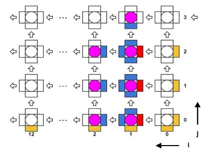
Fig. 5. Scheme of pipeline calculation of tubulin interactions in a microtubule.
It turned out to be possible to realize three complete parallel pipelines capable of updating the coordinates of three molecules each stroke (Fig. 5). Then, in order to avoid idle conveyors, it was necessary to increase the capacity for local memory and to read the coordinates of seven molecules each cycle. This problem was easily solved, practically without changing the original C ++ code, but only through the use of a special directive,
physically breaking down the source dataset on four independent hardware
memory blocks. Since Since BRAM's FPGA is dual-port, of the four memory blocks, you can read 8 values per clock. But, since the three pipelines require the coordinates of 7 molecules per cycle (see Figure 5), this solved the problem.
#pragma HLS DATA_PACK variable=m1, m2 #pragma HLS ARRAY_PARTITION variable=m1, m2 cyclic factor=4 dim=2 | Period | L | II | BRAM | DSP | FF | LUT | Recycling |
|---|---|---|---|---|---|---|---|
| 5 ns | 191 clock | 1 cycle | 52 | 498 | 282550 | 331027 | Absolute |
| 2% | 23% | eleven % | 27% | Relative |
Tab. 1: Performance and disposal of the HLS circuit with three full pipelines
In tab. Figure 1 shows the utilization of the HLS circuit (i.e., the amount of FPGA hardware resources it consumes, in absolute and relative units for a Virtex-7 2000T chip) and its performance. L is the delay or latency of the scheme, i.e. the number of clocks between the first input to the conveyor and the first output is received, II is the initialization interval (or throughput) of the conveyor, meaning after how many clocks the following data can be supplied to the input of the conveyor.
Disposal is given both in absolute values (how many FF triggers or LUT tables are required) for the implementation of the scheme, and in relative to the full amount of this resource in the chip. As can be seen from the table. 1 latency L of a full pipeline was equal to 191 cycles, with each pipeline having to process a third of all molecules, which gives a theoretical estimate of the calculation time for one iteration equal to T (FPGA) = (L + N / 3) * 5ns = 1.2 µs
From tab. Figure 1 also shows that there is still a lot of unused logic in the crystal, but it is impractical to further increase the number of parallel pipelines. Only the second term will decrease, and the initial delay will still make a significant contribution during operation. At the same time, an increase in the amount of logic will complicate the placement and tracing of the circuit in the next stages of project development in Vivado.
Core rand
As mentioned, the algorithm takes into account the Brownian motion of molecules, one of the methods for calculating which is the addition of a normal random additive to the change of coordinates at each iteration over time. You need a lot of normally distributed random numbers, for each iteration - N 3 numbers, which gives the stream 420 10 ^ 6 numbers / s. Such a stream cannot be loaded from the host, so it needs to be generated inside the FPGA on the fly. For this, as in the reference code for the CPU, a Mersenne vortex generator was chosen, giving uniformly distributed pseudo-random numbers. Then a Box-Muller transform was applied to them and normally distributed sequences were obtained at the output. The original open source vortex of Mersenne was modified to obtain a hardware conveyor with an initialization interval of 1 clock. The algorithm requires 9 normal numbers each clock cycle, so the RAND core included 10 independent Mersenn vortex generators, since The Box-Muller transform requires two uniformly distributed numbers to produce 2 normally distributed ones. In tab. 2 shows the utilization of the RAND kernel.
| BRAM | DSP | FF | LUT | Recycling |
|---|---|---|---|---|
| thirty | 41 | 48395 | 64880 | Absolute |
| 1.2% | 9 % | 0.1% | 5.3% | Relative |
Tab. 2: Dispose of the RAND kernel
It can be seen that such a core requires a significant part of the DSP crystal resources, and it would be difficult to place this core in the same SLR with the MT core, since the sum of utilization of two cores at least in DSP resource is 31% more than one SLR can hold (25%).
You can read more about how we chose a pseudo-random number generator and synthesized it in Vivado HLS in the article of my colleague https://habrahabr.ru/post/266897/
Create bitstream
After the integration of computational cores in Vivado, the project imposed spatial restrictions on the placement of IP blocks. The used FPGA Virtex-7 2000T has 4 independent silicon crystals (SLR0, SLR1, SLR2, SLR3). , MT SLR, (pBlock): pBloch_hls MT pBlock_base (. 3). pBlock_hls SLR0 SLR1, pBock_base – SLR2. , , ( SLR) .
, , .
Board Support Package (PCIe core, DDR3 Interface, Internal AXI Bus), — MT HLS , — RAND.
results
Performance
(CPU, GPU FPGA) . 10^7 , . GPU FPGA - .
. , , CPU 1. . 3, , – .
| Platform | , | Performance |
|---|---|---|
| CPU | 22 | one |
| GPU | 14 | 1.6 |
| FPGA | 1.3 | 17 |
Tab. 3:
, GPU CPU 1.6 , FPGA CPU 17 . , FPGA GPU 11 . FPGA 1.3 1.2 - PCI Express.
Energy efficiency
. CPU – Intel Power Gadget. GPU — Nvidia-smi. FPGA – - , RB-8V7. . 4.
| Platform | Power, W | Ex | Ex_rel |
|---|---|---|---|
| CPU | 89.6 | 0.011 | one |
| GPU | 67 | 0.023 | 2 |
| FPGA | 9.6 | 1.77 | 160 |
Tab. 4:
, . ( ) , :
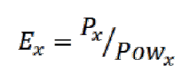
, :
, x = {CPU, GPU, FPGA}.
, FPGA , FPGA . , FPGA .
Discussion
FPGA [12]–[17]. CAAD , ProcStar-III ( Gidel), FPGA Altera Stratix-III SE260. PCI Express -. , 26 CPU Apoal. [24] LAMMPS FPGA. . , . Maxwell, Intel Xeon FPGA Xilinx Virtex-4 [25]. , Maxwell. , 13 . - , CPU SDRAM, FPGA 96% . , , 8-9 .
FPGA . - , FPGA 17 CPU 11 GPU. . , .
FPGA . , .
FPGA . , [26] RTL . , Altera Xilinx (Altera SDK for OpenCL Xilinx Vivado HLS). C/C++ (Xilinx) OpenCL (Altera) . , FPGA [27]–[29]. , [28] Vivado HLS Xilinx Zynq-7000. CPU, 7 . , HLS RTL . Vivado HLS , FPGA. FPGA .
, ! pdf- ,
')
Source: https://habr.com/ru/post/314296/
All Articles