Deep Learning for Newbies: Recognize Handwritten Numbers

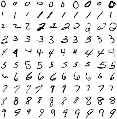
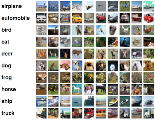
Introducing the first article in the series, conceived to help quickly understand the technology of deep learning ; we will move from basic principles to non-trivial features in order to get decent performance on two data sets: MNIST (handwritten classification) and CIFAR-10 (classification of small images into ten classes: airplane, car, bird, cat, deer, dog, frog , horse, ship and truck).

Intensive development of machine learning technologies has led to the emergence of several very convenient frameworks that allow us to quickly design and build prototypes of our models, as well as provide unlimited access to the data sets used to test learning algorithms (such as those mentioned above). The development environment we will use here is called Keras ; I found it most convenient and intuitive, but at the same time possessing expressive possibilities, sufficient to make changes to the model if necessary.

At the end of this lesson, you will understand the principle of how a simple deep learning model, called a “multilayer perceptron” (MLP), will work, and also learn how to build it in Keras, getting a decent degree of accuracy on MNIST. In the next lesson, we will analyze methods for solving more complex problems of image classification (such as CIFAR-10).

(Artificial) Neurons

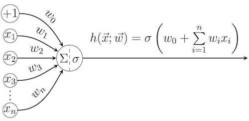
Although the term “deep learning” can be understood in a wider sense, in most cases it is used in the field of (artificial) neural networks . The idea of ​​these constructions is borrowed from biology: neural networks mimic the process of processing of images perceived from the environment by the neurons of the brain and the participation of these neurons in decision making. The principle of operation of a single artificial neuron is essentially very simple: it calculates a weighted sum of all elements of the input vector using the weights vector (as well as the additive component of the displacement ), and then the activation function σ can be applied to the result.

Among the most popular activation features:

• The identity function (Identity): σ ( z ) = z ;
• Sigmoidal function, namely, logistic function (Logistic): and hyperbolic tangent (Tanh):
• Semilinear function (Rectified linear, ReLU)

Initially (from the 1950s), perceptron models were completely linear, that is, only identity served as an activation function. But it soon became clear that the main tasks were often of a non-linear nature, which led to the appearance of other activation functions. Sigmoidal functions (owing their name to the characteristic S-shaped graphics) well simulate the initial “uncertainty” of a neuron regarding a binary solution when z is close to zero, combined with rapid saturation when z is shifted in any direction. The two functions presented here are very similar, but the output values ​​of the hyperbolic tangent belong to the segment [-1, 1], and the range of values ​​of the logistic function is [0, 1] (thus, the logistic function is more convenient for representing the probabilities).

In recent years, semilinear functions and their variations have become widespread in deep learning - they appeared as a simple way to make a model nonlinear (“if the value is negative, nullify it”), but in the end it turned out to be more successful than the historically more popular sigmoidal functions, moreover, they are more consistent with the way a biological neuron transmits an electrical impulse. For this reason, in this lesson we will focus on semilinear functions (ReLU).

Each neuron is uniquely determined by its weight vector. and the main goal of the learning algorithm is to assign a set of weights to a neuron on the basis of a training sample of known pairs of input and output data in order to minimize the prediction error. A typical example of such an algorithm is the gradient descent method, which for a specific loss function changes the weight vector in the direction of the greatest decrease of this function:

where η is a positive parameter, called the learning rate .

The loss function reflects our understanding of how imprecise a neuron is in making decisions for the current value of the parameters. The simplest choice of the loss function, which is good for most problems, is a quadratic function ; for a given training sample it is defined as the square of the difference between the target value y and the actual output value of the neuron for a given input :

The network has a large number of training courses that look at gradient descent algorithms in more depth. In our case, the framework will take care of all the optimization for us, so I will not pay much attention to it in the future.

Introduction to Neural Networks (and Deep Learning)

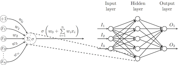
Now that we have introduced the concept of a neuron, it becomes possible to connect the output of one neuron with the input of another, thus marking the beginning of a neural network . In general, we will focus our attention on direct propagation neural networks in which neurons form layers in such a way that the neurons of one layer process the output of the previous layer. In the most powerful of these architectures ( multilayer perceptrons , MLP), all the output of one layer is connected to all the neurons of the next layer, as in the diagram below.

To change the weights of the output neurons, the gradient descent method described above with a given loss function can be directly used; for other neurons, these losses must be propagated in the opposite direction (using the differentiation rule of a complex function), thus initiating the backpropagation algorithm . Just as with the gradient descent method, I will not pay attention to the mathematical substantiation of the algorithm, since all the calculations are performed by our framework.

According to the universal approximation theorem Tsybenko, a sufficiently wide multilayer perceptron with one hidden layer of sigmoidal neurons can approximate any continuous function of real variables on a given interval. The proof of this theorem has no practical application and does not offer an effective training algorithm for such structures. The answer gives deep learning: instead of width, increase depth ; By definition, any neural network with more than one hidden layer is considered deep.

Displacement also allows us to input raw input to the neural network: in the past, single-layer networks were fed with key features ( features ) that were extracted from the input data using special functions. This meant that different classes of tasks, such as computer vision , speech recognition, or the processing of natural languages , required different approaches, which hampered scientific collaboration between these areas. But when the network contains several hidden layers, it acquires the ability to learn to select the key features that best describe the input data, thus finding end-to-end learning (without the traditional programmable processing between input and output), as well as allowing you to use one the same network for a wide range of tasks , since it is no longer necessary to derive functions for obtaining key features. I will give a graphic confirmation of the above in the second part of the lecture, when we consider convolutional neural networks.

Apply Deep MLP to MNIST

Now we will implement the simplest possible deep neural network - MLP with two hidden layers - and apply it to the problem of recognizing handwritten numbers from the MNIST data set.

Only the following imports are required:

from keras.datasets import mnist # subroutines for fetching the MNIST dataset from keras.models import Model # basic class for specifying and training a neural network from keras.layers import Input, Dense # the two types of neural network layer we will be using from keras.utils import np_utils # utilities for one-hot encoding of ground truth values 

Then we define some parameters of our model. These parameters are often referred to as hyperparameters , since they are expected to be refined even before the start of training. In this guide, we take the pre-selected values, the process of clarifying them will pay more attention in subsequent lessons.

In particular, we define:
batch_size - the number of training samples processed simultaneously in one iteration of the gradient descent algorithm;
num_epochs - the number of iterations of the learning algorithm over the entire training set;
hidden_size is the number of neurons in each of the two hidden MLP layers.

 batch_size = 128 # in each iteration, we consider 128 training examples at once num_epochs = 20 # we iterate twenty times over the entire training set hidden_size = 512 # there will be 512 neurons in both hidden layers 

It's time to download MNIST and do some preliminary processing. With Keras, this is done very simply: it simply reads data from a remote server directly into the NumPy library arrays.

To prepare the data, we first present the images as one-dimensional arrays (since we consider each pixel as a separate input feature), and then divide the intensity value of each pixel by 255 so that the new value falls into the [0, 1] segment. This is a very simple way to normalize the data, we will discuss other ways in subsequent lessons.

A good approach to the classification problem is a probabilistic classification , in which we have one output neuron for each class, which gives the probability that the input element belongs to this class. This implies the need to convert the training output into direct encoding: for example, if the desired output class is 3 and there are five classes in total (and they are numbered from 0 to 4), then suitable direct encoding is [0, 0, 0, 1, 0] . Again, Keras offers us all this functionality out of the box.

 num_train = 60000 # there are 60000 training examples in MNIST num_test = 10000 # there are 10000 test examples in MNIST height, width, depth = 28, 28, 1 # MNIST images are 28x28 and greyscale num_classes = 10 # there are 10 classes (1 per digit) (X_train, y_train), (X_test, y_test) = mnist.load_data() # fetch MNIST data X_train = X_train.reshape(num_train, height * width) # Flatten data to 1D X_test = X_test.reshape(num_test, height * width) # Flatten data to 1D X_train = X_train.astype('float32') X_test = X_test.astype('float32') X_train /= 255 # Normalise data to [0, 1] range X_test /= 255 # Normalise data to [0, 1] range Y_train = np_utils.to_categorical(y_train, num_classes) # One-hot encode the labels Y_test = np_utils.to_categorical(y_test, num_classes) # One-hot encode the labels 

And now the time has come to determine our model! To do this, we will use a stack of three Dense layers, which corresponds to a fully connected MLP, where all the outputs of one layer are connected to all the inputs of the next. We will use ReLU for the neurons of the first two layers, and softmax for the last layer. This activation function is designed to transform any vector with real values ​​into a probability vector and is defined for the jth neuron as follows:

Keras's remarkable feature that distinguishes it from other frameworks (for example, from TansorFlow) is the automatic calculation of layer sizes; we only need to specify the dimension of the input layer, and Keras automatically initializes all other layers. When all layers are defined, we just need to set the input and output data, as is done below.

 inp = Input(shape=(height * width,)) # Our input is a 1D vector of size 784 hidden_1 = Dense(hidden_size, activation='relu')(inp) # First hidden ReLU layer hidden_2 = Dense(hidden_size, activation='relu')(hidden_1) # Second hidden ReLU layer out = Dense(num_classes, activation='softmax')(hidden_2) # Output softmax layer model = Model(input=inp, output=out) # To define a model, just specify its input and output layers 

Now we just need to determine the loss function, the optimization algorithm and the metrics that we will collect.

When dealing with a probabilistic classification, it’s best to use as a loss function the quadratic error not defined above, but the cross entropy. For a certain output probability vector compared to the actual vector loss (for the k- th class) will be defined as

Losses will be less for probabilistic tasks (for example, with a logistic / softmax function for the output layer), mainly due to the fact that this function is designed to maximize the confidence of the model in the correct class definition, and it does not care about the probability distribution of the sample to other classes (while the quadratic error function tends to ensure that the probability of hitting the other classes is as close to zero as possible).

The optimization algorithm used will resemble some form of the gradient descent algorithm, the only difference being in how the learning rate η is chosen. An excellent overview of these approaches is presented here , and now we will use Adam's optimizer, which usually shows good performance.

Since our classes are balanced (the number of handwritten numbers belonging to each class is the same), accuracy will be a suitable metric - the proportion of input data assigned to the correct class.

 model.compile(loss='categorical_crossentropy', # using the cross-entropy loss function optimizer='adam', # using the Adam optimiser metrics=['accuracy']) # reporting the accuracy 

Finally, we run the learning algorithm. It is good practice to set aside some subset of data to verify that our algorithm (still) correctly recognizes the data — this data is also called the validation set ; here we separate 10% of the data for this purpose.

Another nice feature of Keras is the granularity: it displays detailed logging of all steps of the algorithm.

 model.fit(X_train, Y_train, # Train the model using the training set... batch_size=batch_size, nb_epoch=num_epochs, verbose=1, validation_split=0.1) # ...holding out 10% of the data for validation model.evaluate(X_test, Y_test, verbose=1) # Evaluate the trained model on the test set! 

 Train on 54000 samples, validate on 6000 samples Epoch 1/20 54000/54000 [==============================] - 9s - loss: 0.2295 - acc: 0.9325 - val_loss: 0.1093 - val_acc: 0.9680 Epoch 2/20 54000/54000 [==============================] - 9s - loss: 0.0819 - acc: 0.9746 - val_loss: 0.0922 - val_acc: 0.9708 Epoch 3/20 54000/54000 [==============================] - 11s - loss: 0.0523 - acc: 0.9835 - val_loss: 0.0788 - val_acc: 0.9772 Epoch 4/20 54000/54000 [==============================] - 12s - loss: 0.0371 - acc: 0.9885 - val_loss: 0.0680 - val_acc: 0.9808 Epoch 5/20 54000/54000 [==============================] - 12s - loss: 0.0274 - acc: 0.9909 - val_loss: 0.0772 - val_acc: 0.9787 Epoch 6/20 54000/54000 [==============================] - 12s - loss: 0.0218 - acc: 0.9931 - val_loss: 0.0718 - val_acc: 0.9808 Epoch 7/20 54000/54000 [==============================] - 12s - loss: 0.0204 - acc: 0.9933 - val_loss: 0.0891 - val_acc: 0.9778 Epoch 8/20 54000/54000 [==============================] - 13s - loss: 0.0189 - acc: 0.9936 - val_loss: 0.0829 - val_acc: 0.9795 Epoch 9/20 54000/54000 [==============================] - 14s - loss: 0.0137 - acc: 0.9950 - val_loss: 0.0835 - val_acc: 0.9797 Epoch 10/20 54000/54000 [==============================] - 13s - loss: 0.0108 - acc: 0.9969 - val_loss: 0.0836 - val_acc: 0.9820 Epoch 11/20 54000/54000 [==============================] - 13s - loss: 0.0123 - acc: 0.9960 - val_loss: 0.0866 - val_acc: 0.9798 Epoch 12/20 54000/54000 [==============================] - 13s - loss: 0.0162 - acc: 0.9951 - val_loss: 0.0780 - val_acc: 0.9838 Epoch 13/20 54000/54000 [==============================] - 12s - loss: 0.0093 - acc: 0.9968 - val_loss: 0.1019 - val_acc: 0.9813 Epoch 14/20 54000/54000 [==============================] - 12s - loss: 0.0075 - acc: 0.9976 - val_loss: 0.0923 - val_acc: 0.9818 Epoch 15/20 54000/54000 [==============================] - 12s - loss: 0.0118 - acc: 0.9965 - val_loss: 0.1176 - val_acc: 0.9772 Epoch 16/20 54000/54000 [==============================] - 12s - loss: 0.0119 - acc: 0.9961 - val_loss: 0.0838 - val_acc: 0.9803 Epoch 17/20 54000/54000 [==============================] - 12s - loss: 0.0073 - acc: 0.9976 - val_loss: 0.0808 - val_acc: 0.9837 Epoch 18/20 54000/54000 [==============================] - 13s - loss: 0.0082 - acc: 0.9974 - val_loss: 0.0926 - val_acc: 0.9822 Epoch 19/20 54000/54000 [==============================] - 12s - loss: 0.0070 - acc: 0.9979 - val_loss: 0.0808 - val_acc: 0.9835 Epoch 20/20 54000/54000 [==============================] - 11s - loss: 0.0039 - acc: 0.9987 - val_loss: 0.1010 - val_acc: 0.9822 10000/10000 [==============================] - 1s [0.099321320021623111, 0.9819] 

As you can see, our model achieves an accuracy of approximately 98.2% on a test dataset, which is quite worthy for such a simple model, despite the fact that it is far surpassed by the cutting-edge approaches described here .

I urge you to experiment with this model: try various hyperparameters, optimization algorithms, activation functions, add hidden layers, etc. In the end, you should be able to achieve accuracy above 99%.

Conclusion

In this post, we covered the basic concepts of deep learning, successfully implemented a simple two-layer deep MLP using the Keras framework, applied it to the MNIST data set — all in less than 30 lines of code.

Next time, we will look at convolutional neural networks (CNN), which solve some of the problems that arise when applying MLP to large-scale images (such as CIFAR-10).