Optimal Spline Approximation
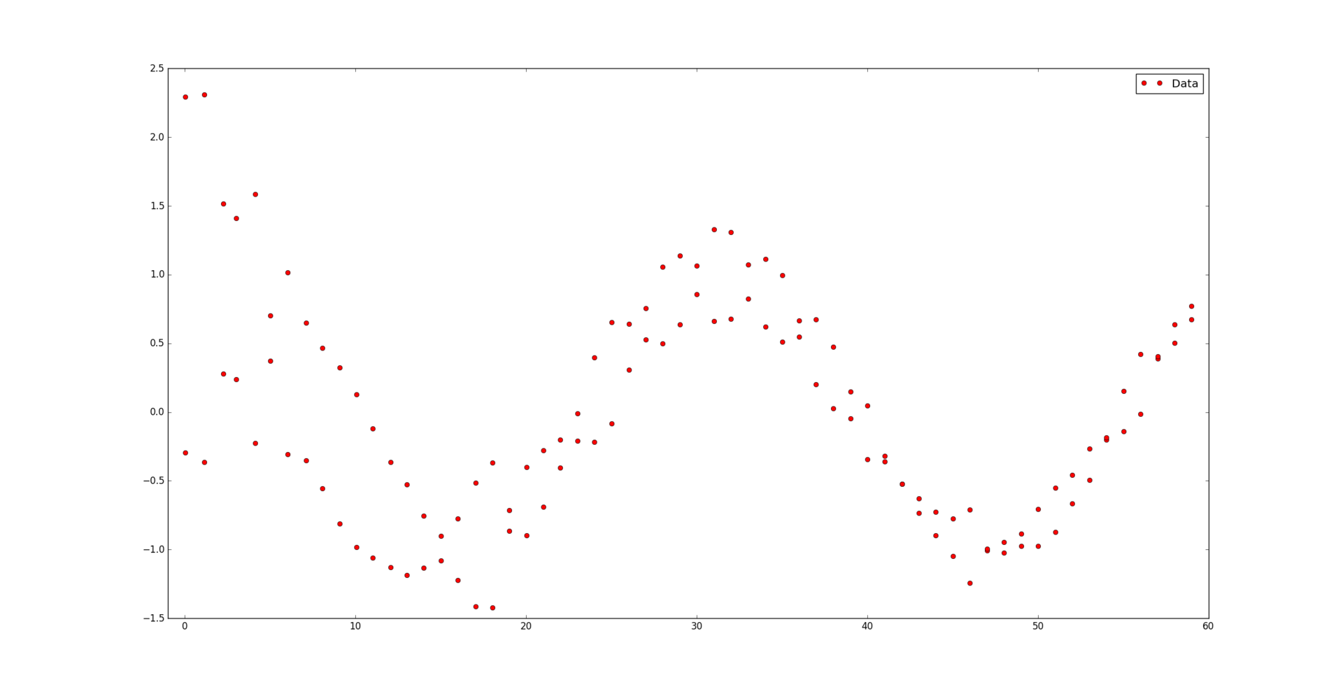
Let us be given a set of points  and the corresponding set of positive weights
  . We believe that some points may be more important than others (if not, then all the weights are the same). Informally speaking, we want a beautiful curve to be drawn at the appropriate interval so that it “best of all” passes through this data.
Under the cat is an algorithm that reveals how the splines allow you to build such a beautiful regression, as well as its implementation in Python :
The function s (x) on the interval [a, b] is called a spline of degree k on a grid with horizontal nodes if the following properties are true:
Note that to build a spline, you first need to create a grid of horizontal nodes. Arrange them in such a way that within the interval (a, b) there are g nodes, and at the edges - k + 1: and
and  .
.
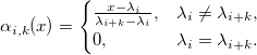
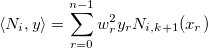
Every spline at point can be presented in basic form:
')

Where - B-spline k + 1st order :


Here's how, for example, looks like a basis on a grid of g = 9 nodes, evenly distributed on the interval [0, 1]:

Immediately understand the construction of splines through B-splines is very difficult. More information can be found here .
So, we found out that the spline is determined uniquely by nodes and coefficients. Assume that the nodes we are known. Also at the entrance is a set of data with appropriate weights . It is necessary to find the coefficients  approximating the spline curve to the data. Strictly speaking, they must deliver a minimum of function.

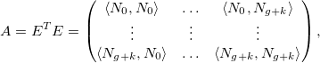
For convenience, we write in matrix form:

Where


Note that the matrix E is block-diagonal. The minimum is reached when the gradient of the error in the coefficients is zero:

Set the operator denoting a weighted scalar product:
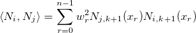
Let also

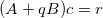
Then the whole task and all previous formulas are reduced to solving a simple system of linear equations:

where matrix A is (2k + 1) -diagonal, since if | i - j | > k. Also, matrix A is symmetric and positive-definite, hence the solution can be quickly found using the Cholesky decomposition (there is also an algorithm for sparse matrices).
And so, solving the system, we get the desired result:
However, everything is not always so good. With a small amount of data in relation to the number of nodes and the degree of the spline, a so-called problem may arise. overfitting. Here is an example of a “bad” cubic spline, while ideally passing through the data:
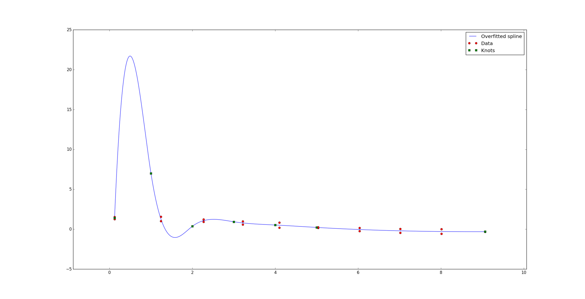
OK, the curve is not so beautiful anymore. We will try to reduce the so-called oscillations of the spline. To do this, we will try to “smooth out” its kth derivative. In other words, we minimize the difference between the derivative to the left and the derivative to the right of each node:
Expanding the spline in the basic form, we get:

Let's look at the error

Here q is the weight of the function that affects smoothing, and
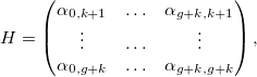

New system of equations:
Where

The rank of matrix B is g. It is symmetric and, since q> 0, A + qB will be positive definite. Therefore, the Cholesky decomposition is still applicable to the new system of equations. However, the matrix B is degenerate and if q values are too large, numerical errors may occur.
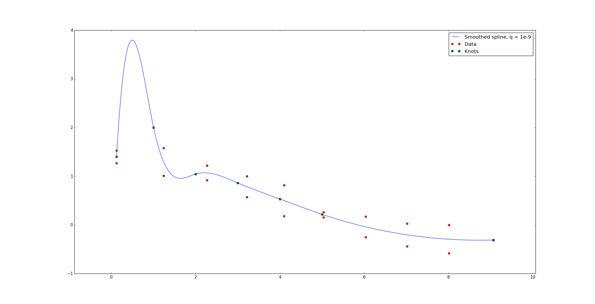
For a very small value of q = 1e-9, the shape of the curve changes very little.
But at q = 1e-7 in this example, sufficient smoothing is already achieved.

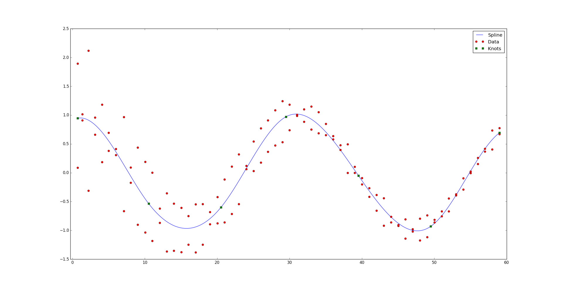
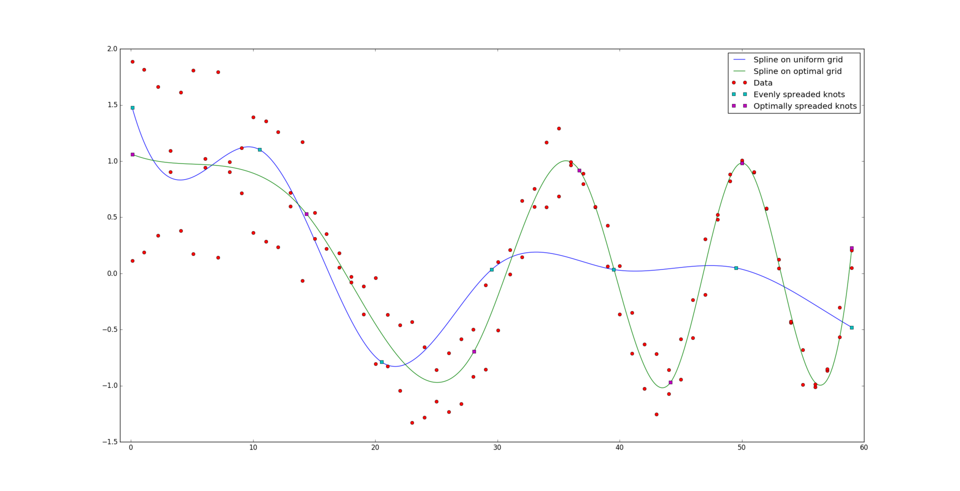
Imagine now that the task is the same as before, except that we do not know how the nodes are located on the grid. Apart from the data, only the number of nodes g, the interval [a, b] and the degree of the spline k are fed to the input. Let us naively assume that it is best to arrange the nodes evenly on the interval:

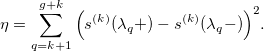
Oops. Apparently, it is necessary to position the nodes somehow differently. Formally, arrange the nodes so that the error value

was minimal. The last term plays the role of the penalty function so that the nodes do not closely approach each other:
The positive parameter p is the weight of the penalty function. The greater its value, the faster the nodes will move away from each other and tend to a uniform location.
To solve this problem, we use the conjugate gradient method. Its charm lies in the fact that for a quadratic function it converges in a fixed (in this case, g) number of steps.
To find the value minimum function

we use an algorithm that allows us to reduce the number of calls to the oracle, namely the number of approximation operations with given nodes and the calculation of the error function. We will use the notation .
.
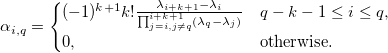
The coefficients a i and b i can be found from the equations

and

Explanation of the algorithm:
The idea is to arrange three points α 0 <α 1 <α 2 in such a way that a simple approximating function can be constructed from the error values achieved at these points and return its minimum. Moreover, the error value in α 1 must be less than the error value in α 0 and α 2 .
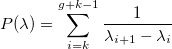
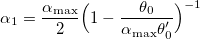
Find the initial approximation α 1 from the condition S '(α 1 ) = 0, where S (α) is a function of the form
The constants c 0 and c 1 are found from the conditions and
and  .
.
If we miscalculated with the initial approximation, then we decrease the step α 1 as long as it delivers a larger error value than α 0 . Selection proceeds from the condition
  where Q (α) is the parabola interpolating error function
  :
:  ,
,  and
and  .
.
If k> 0, then we have found the value of α 1 , such that when choosing it, the error value will be less than when choosing α 0 and α 2 , and we return it as a rough approximation of α *.
If our initial approximation was correct, then we are trying to find a step α 2 such that . It will be found between α 1 and α max , since α max is the singularity point for the penalty function.
When all three α 0 , α 1 and α 2 values are found, we represent the error function as the sum of two functions approximating the difference of squares and the penalty function. The function Q (α) is a parabola whose coefficients can be found, since we know its values at three points. The function R (α) goes to infinity as α tends to α max . The coefficients b i can also be found from a system of three equations. As a result, we arrive at an equation that can be quadratic and easily solved:

And so, for comparison, the result of an optimally constructed spline:
Well and for those to whom it can be useful: implementation on Python .
and the corresponding set of positive weights . We believe that some points may be more important than others (if not, then all the weights are the same). Informally speaking, we want a beautiful curve to be drawn at the appropriate interval so that it “best of all” passes through this data.Under the cat is an algorithm that reveals how the splines allow you to build such a beautiful regression, as well as its implementation in Python :
Basic definitions
The function s (x) on the interval [a, b] is called a spline of degree k on a grid with horizontal nodes
if the following properties are true:- At intervals
 The function s (x) is a kth power polynomial.
 - The n-th derivative of the function s (x) is continuous at any point [a, b] for any n = 1, ..., k-1.
Note that to build a spline, you first need to create a grid of horizontal nodes. Arrange them in such a way that within the interval (a, b) there are g nodes, and at the edges - k + 1:
and .Every spline at point
can be presented in basic form:')
Where
- B-spline k + 1st order :Here's how, for example, looks like a basis on a grid of g = 9 nodes, evenly distributed on the interval [0, 1]:
Immediately understand the construction of splines through B-splines is very difficult. More information can be found here .
Approximation with given horizontal nodes
So, we found out that the spline is determined uniquely by nodes and coefficients. Assume that the nodes
we are known. Also at the entrance is a set of data with appropriate weights . It is necessary to find the coefficients approximating the spline curve to the data. Strictly speaking, they must deliver a minimum of function.For convenience, we write in matrix form:
Where
Note that the matrix E is block-diagonal. The minimum is reached when the gradient of the error in the coefficients is zero:
Set the operator
denoting a weighted scalar product:Let also
Then the whole task and all previous formulas are reduced to solving a simple system of linear equations:
where matrix A is (2k + 1) -diagonal, since
if | i - j | > k. Also, matrix A is symmetric and positive-definite, hence the solution can be quickly found using the Cholesky decomposition (there is also an algorithm for sparse matrices).And so, solving the system, we get the desired result:
Smoothing
However, everything is not always so good. With a small amount of data in relation to the number of nodes and the degree of the spline, a so-called problem may arise. overfitting. Here is an example of a “bad” cubic spline, while ideally passing through the data:
OK, the curve is not so beautiful anymore. We will try to reduce the so-called oscillations of the spline. To do this, we will try to “smooth out” its kth derivative. In other words, we minimize the difference between the derivative to the left and the derivative to the right of each node:
Expanding the spline in the basic form, we get:
Let's look at the error
Here q is the weight of the function that affects smoothing, and
New system of equations:
Where
The rank of matrix B is g. It is symmetric and, since q> 0, A + qB will be positive definite. Therefore, the Cholesky decomposition is still applicable to the new system of equations. However, the matrix B is degenerate and if q values are too large, numerical errors may occur.
For a very small value of q = 1e-9, the shape of the curve changes very little.
But at q = 1e-7 in this example, sufficient smoothing is already achieved.
Approximation with unknown horizontal nodes
Imagine now that the task is the same as before, except that we do not know how the nodes are located on the grid. Apart from the data, only the number of nodes g, the interval [a, b] and the degree of the spline k are fed to the input. Let us naively assume that it is best to arrange the nodes evenly on the interval:
Oops. Apparently, it is necessary to position the nodes somehow differently. Formally, arrange the nodes so that the error value
was minimal. The last term plays the role of the penalty function so that the nodes do not closely approach each other:
The positive parameter p is the weight of the penalty function. The greater its value, the faster the nodes will move away from each other and tend to a uniform location.
To solve this problem, we use the conjugate gradient method. Its charm lies in the fact that for a quadratic function it converges in a fixed (in this case, g) number of steps.
- Initialize the direction
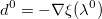 .How to calculate the derivative of the error on the nodes?The derivative of the sum of squares by node:
In order to calculate the influence of the position of the node on the values of the spline, it is necessary to consider the B-splines. on new nodes
  and with new coefficients


Derivative of the penalty function:
You can’t look at the derivative smoothing function without tears:
- For j = 0, ..., g-1
- Set the function
returning an error depending on the choice of step along a given direction. At this step, we find the optimal value of α * that delivers the minimum of this function. To do this, we solve the problem of one-dimensional optimization. How it will be discussed later. - Update node values:

- Update the direction vector:

- Set the function
- If a
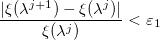
and
where ε 1 and ε 2 are predetermined values that are responsible for the accuracy of the algorithm, then we exit. Otherwise, reset the counter and return to the first step.
Solving the problem of one-dimensional minimization
To find the value
minimum functionwe use an algorithm that allows us to reduce the number of calls to the oracle, namely the number of approximation operations with given nodes and the calculation of the error function. We will use the notation
.- Let the first and last components of the direction vector be zero:
 . We will also set the maximum possible step along this direction:
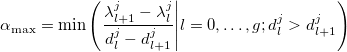
This choice is due to the fact that the nodes should not intersect. - Initiate k = 0 and initial steps:
 ,
,  ,
,  .
. - Until
 :
:- Ask

and reduce the step
- k = k + 1
- Ask
- If k> 0, then we return α * = α 1 . Otherwise:
- Until
 : α 0 = α 1 , α 1 = α 2 and
- Return
 where
where  - the root of the equation I '(α) = 0 and I (α) - approximation of the error function:
Where

- Until
The coefficients a i and b i can be found from the equations
and
Explanation of the algorithm:
The idea is to arrange three points α 0 <α 1 <α 2 in such a way that a simple approximating function can be constructed from the error values achieved at these points and return its minimum. Moreover, the error value in α 1 must be less than the error value in α 0 and α 2 .
Find the initial approximation α 1 from the condition S '(α 1 ) = 0, where S (α) is a function of the form
The constants c 0 and c 1 are found from the conditions
and .If we miscalculated with the initial approximation, then we decrease the step α 1 as long as it delivers a larger error value than α 0 . Selection
proceeds from the condition where Q (α) is the parabola interpolating error function : , and .If k> 0, then we have found the value of α 1 , such that when choosing it, the error value will be less than when choosing α 0 and α 2 , and we return it as a rough approximation of α *.
If our initial approximation was correct, then we are trying to find a step α 2 such that
. It will be found between α 1 and α max , since α max is the singularity point for the penalty function.When all three α 0 , α 1 and α 2 values are found, we represent the error function as the sum of two functions approximating the difference of squares and the penalty function. The function Q (α) is a parabola whose coefficients can be found, since we know its values at three points. The function R (α) goes to infinity as α tends to α max . The coefficients b i can also be found from a system of three equations. As a result, we arrive at an equation that can be quadratic and easily solved:
And so, for comparison, the result of an optimally constructed spline:
Well and for those to whom it can be useful: implementation on Python .
Source: https://habr.com/ru/post/314218/
All Articles