[Bookmark] Zoo neural network architectures. Part 2
We publish the second part of the article about the types of neural network architecture. Here is the first.
It is not easy to keep track of all the neural network architectures that continually arise lately. Even understanding all the abbreviations that professionals throw at first may seem like an impossible task.
')
Therefore, I decided to make a cheat sheet for such architectures. Most of them are neural networks, but some are animals of a different breed. Although all these architectures are presented as new and unique, when I portrayed their structure, internal communications have become much clearer.
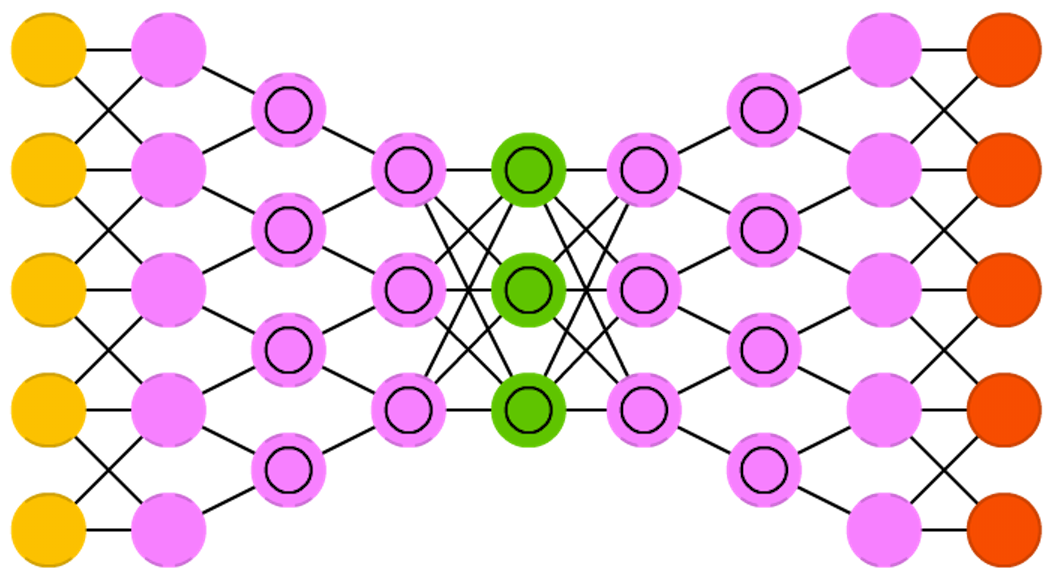
The name “ Deep convolutional inverse graphics networks (DCIGN) " can be misleading, because in reality these are variational autoencoders with convolutional and sweeping networks as encoding and decoding parts, respectively. Such networks present image features as probabilities and can learn how to build an image of a cat and a dog together, looking only at the pictures with cats and only with dogs. In addition, you can show this network a photo of your cat with an annoying neighbor the dog and ask her to cut the dog and the images, and DCIGN will cope with this task, even if it has never done anything like that. The developers also demonstrated that DCIGN can simulate various complex image transformations, such as changing the light source or rotating 3D objects. teach the method of back propagation.
Kulkarni, Tejas D., et al. “Deep convolutional inverse graphics network.” Advances in Neural Information Processing Systems. 2015
Original Paper PDF
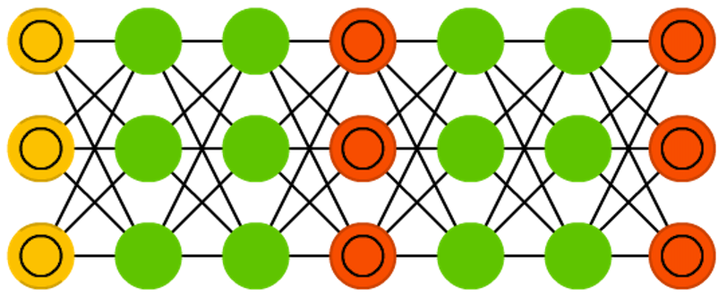
Generative adversarial networks (GAN) belong to another family of neural networks, these are twins - two networks working together. A GAN consists of any two networks (but more often it is a direct distribution or convolutional network), where one of the networks generates data (“generator”), and the second analyzes (“discriminator”). The discriminator receives input or training data, or generated by the first network. How accurately the discriminator will be able to determine the source of the data is then used to estimate generator errors. Thus, a kind of competition takes place, where the discriminator learns to better distinguish real data from the generated ones, and the generator tends to become less predictable for the discriminator. This works in part because even complex images with a lot of noise eventually become predictable, but the generated data, which is little different from the real ones, is more difficult to learn to distinguish. GAN is quite difficult to train, since the task here is not just to train the two networks, but also to observe the necessary balance between them. If one of the parts (generator or discriminator) becomes much better than the other, then the GAN will never converge.
Goodfellow, Ian, et al. “Generative adversarial nets.” Advances in Neural Information Processing Systems. 2014
Original Paper PDF

Recurrent neural networks (Recurrent neural networks, RNN) are the same networks of direct distribution, but with a shift in time: neurons receive information not only from the previous layer, but also from themselves as a result of the previous passage. Therefore, the order in which we submit information and train the network is important: we will get different results if we feed her “milk” first, and then “cookies”, or if we get “cookies” first, and then “milk”. RNN has one big problem - the problem of a vanishing (or explosive) gradient: depending on the activation function used, information is lost over time, as well as in very deep direct propagation networks. It would seem that this is not such a serious problem, since it concerns only the weights, not the states of the neurons, but it is in the scales that information about the past is stored; if the weight reaches a value of 0 or 1,000,000, then the information about the past state will not be too informative. RNNs can be used in a wide variety of areas, since even data not related to the passage of time (not audio or video) can be represented as a sequence. A picture or a line of text can be fed to the input one pixel or one character, so the weight will be used for the previous element of the sequence, and not for what happened X seconds ago. In general, recurrent networks are good for continuing or supplementing information, for example, autocompletion.
Elman, Jeffrey L. “Finding structure in time.” Cognitive science 14.2 (1990): 179-211.
Original Paper PDF

Long short term memory (LSTM) - an attempt to overcome the problem of explosive gradient, using filters (gates) and memory blocks (memory cells). This idea came, rather, from the field of circuit design, rather than biology. Each neuron has three filters: an input filter (input gate), an output filter (output gate) and a forgetting filter (forget gate). The task of these filters is to save information, stopping and resuming its flow. The input filter determines the amount of information from the previous step that will be stored in the memory block. The output filter is busy determining how much information the next layer will receive about the current state of the node. The presence of the forgetting filter at first glance seems strange, but sometimes it turns out to be useful to forget: if the neural network remembers a book, at the beginning of a new chapter it may be necessary to forget some of the characters from the previous one. It has been shown that LSTM can learn really complex sequences, for example, to imitate Shakespeare or compose simple music. It should be noted that since each filter keeps its weight relative to the previous neuron, such networks are quite resource-intensive.
Hochreiter, Sepp, and Jürgen Schmidhuber. “Long short-term memory.” Neural computation 9.8 (1997): 1735-1780.
Original Paper PDF

Managed recurrent neurons (Gated recurrent units, GRU) are a type of LSTM. They have one less filter, and they are slightly differently connected: instead of the input, output filters and forgetting filters, the update gate is used here. This filter determines how much information to save from the last state, and how much information to get from the previous layer. The reset gate filter works almost the same as the forgetting filter, but is located a little differently. Full status information is sent to the next layers — there is no output filter here. In most cases, GRUs work just like LSTM, the most significant difference is that the GRUs are slightly faster and easier to operate (however, they have slightly less expressive capabilities).
Chung, Junyoung, et al. “Empirical evaluation of recurrent neural networks on sequence modeling.” ArXiv preprint arXiv: 1412.3555 (2014).
Original Paper PDF

Neural Turing machines (NMT) can be defined as an abstraction over LSTM and an attempt to “get” the neural network from the black box, giving us an idea of what is happening inside. The memory block here is not built into the neuron, but is separated from it. This allows you to combine the performance and immutability of the usual digital data storage with the performance and expressive capabilities of the neural network. The idea is to use addressable memory and neural networks, which can read from this memory and write to it. They are called Turing neural machines, since they are Turing-complete: the ability to read, write, and change state based on what you read allows you to do everything that a universal Turing machine can do.
Graves, Alex, Greg Wayne, and Ivo Danihelka. “Neural turing machines.” ArXiv preprint arXiv: 1410.5401 (2014).
Original Paper PDF
Bidirectional RNN, LSTM and GRU (BiRNN, BiLSTM and BiGRU) are not shown in the diagram, as they look exactly the same as their unidirectional counterparts. The only difference is that these neural networks are connected not only with the past, but also with the future. For example, a unidirectional LSTM can learn to predict the word “fish” by receiving letters one at a time. Bidirectional LSTM will also receive the next letter during the back pass, thus opening access to future information. This means that a neural network can be trained not only to supplement information, but also to fill in gaps, so, instead of expanding the pattern along the edges, it can finish drawing missing fragments in the middle.
Schuster, Mike, and Kuldip K. Paliwal. “Bidirectional recurrent neural networks.” IEEE Transactions on Signal Processing 45.11 (1997): 2673-2681.
Original Paper PDF

Deep residual networks (Deep Resualual Networks, DRN) are very deep FFNNs with additional connections between layers, usually two to five, connecting not only adjacent layers, but also more distant ones. Instead of looking for a way to find the input data corresponding to the source data through, say, five layers, the network is trained to match the “output block + input block” pair to the input block. Thus, the input data passes through all layers of the neural network and is served on a platter to the last layers. It was shown that such networks can be trained in patterns with a depth of up to 150 layers, which is much more than can be expected from an ordinary 2-5-layer neural network. However, it has been proven that networks of this type are in fact just RNN without explicit use of time, and they are often compared to LSTM without filters.
He, Kaiming, et al. “Deep residual learning for image recognition.” ArXiv preprint arXiv: 1512.03385 (2015).
Original Paper PDF

Neural echo networks (Echo state networks, ESN) are another type of recurrent neural networks. They stand out because the connections between the neurons in them are random, not organized into neat layers, and they are trained differently. Instead of submitting data to the input and backward propagation of an error, we transmit data, update the state of the neurons, and monitor the output for some time. The input and output layers play a non-standard role, since the input layer serves to initialize the system, and the output layer - as an observer of the order of activation of neurons, which manifests itself with time. During training, only the connections between the observer and the hidden layers change.
Jaeger, Herbert, and Harald Haas. “Harnessing nonlinearity: Predicting chaotic systems and energy saving in wireless communication.” Science 304.5667 (2004): 78-80.
Original Paper PDF

Extreme learning machines (ELM) are the same FFNN, but with random connections between neurons. They are very similar to LSM and ESN, but are used rather like forward-propagation networks, and this is not due to the fact that they are not recurrent or impulsive, but to the fact that they are trained by the back propagation method.
Cambria, Erik, et al. “Extreme learning machines [trends & controversies].” IEEE Intelligent Systems 28.6 (2013): 30-59.
Original Paper PDF

Unstable state machines (Liquid state machines, LSM) are similar to ESNs. Their main difference is that LSM is a kind of impulse neural networks: threshold functions come to replace the sigmoidal curve, and each neuron is also a cumulative memory block. When the state of the neuron is updated, the value is not calculated as the sum of its neighbors, but is added to itself. As soon as the threshold is exceeded, the energy is released and the neuron sends an impulse to other neurons.
Maass, Wolfgang, Thomas Natschläger, and Henry Markram. “A new framework for neural computation based on perturbations.” Neural computation 14.11 (2002): 2531-2560.
Original Paper PDF

The support vector machine (SVM) method is used to find optimal solutions in classification problems. In the classical sense, the method is capable of categorizing linearly shared data: for example, determine which figure shows Garfield, and which figure shows Snoopy. In the process of learning, the network places all Garfields and Snoopy on 2D graphics and tries to divide the data with a straight line so that each side has data of only one class and the distance from the data to the line is maximum. Using a trick with the kernel, one can classify data of dimension n. Having built a 3D graph, we can distinguish Garfield from Snoopy and Simon the cat, and the higher the dimension, the more cartoon characters you can classify. This method is not always considered as a neural network.
Cortes, Corinna, and Vladimir Vapnik. “Support-vector networks.” Machine learning 20.3 (1995): 273-297.
Original Paper PDF

Finally, the last inhabitant of our zoo is the Kohonen networks, KN, or organizing (feature) map, SOM, SOFM map of Kohonen . KN uses competitive training to classify data without a teacher. The network analyzes its neurons for maximum match with the input data. The most suitable neurons are updated so as to even closer look like the input data, in addition, the weights of their neighbors are getting closer to the input data. How much the state of the neighbors changes depends on the distance to the most suitable node. KN is also not always referred to as neural networks.
Kohonen, Teuvo. “Self-organized formation of topologically correct feature maps.” Biological cybernetics 43.1 (1982): 59-69.
Original Paper PDF
Read the first part too.
Source: https://habr.com/ru/post/313906/
All Articles