Tensor expansions and their applications. Lecture in Yandex
The previous lecture with Data Fest was devoted to the algorithms needed to build a new kind of search. Today's report is also in a certain sense about different algorithms, more precisely, about the mathematics that underlies many of them. Ivan Oseledets, Ph.D. and head of the Skoltech computational methods group, told the audience about the matrix expansions.
Under the cut - the decoding and most of the slides.
There is a small - relatively machine learning - community that deals with linear algebra. There is linear algebra, and there are people in it who are engaged in multilinear algebra, tensor decompositions. I treat them. A sufficiently large number of interesting results were obtained there, but due to the ability of the community to self-organize and not go outside, some of these results are unknown. By the way, this also applies to linear algebra. If you look at the articles of the leading conferences of the NIPS, ICML, etc., then you can see quite a lot of articles related to the trivial facts of linear algebra. This happens, but nonetheless.
')
We will talk about tensor expansions, but first we must say about matrix expansions.

Matrices. Just a two-dimensional table. The matrix decomposition is a representation of the matrix in the form of products of Boolean primes. In fact, they are used everywhere, everyone has mobile phones, and while you are sitting, they solve linear systems, transfer data, decompose matrices. True, these matrices are very small - 4x4, 8x8. But in practice, these matrices are very important.
I must say that there is a LU decomposition, Gauss decomposition, QR decomposition, but I will mainly talk about singular decomposition, which for some reason, for example, in linear algebra courses in our universities is undeservedly forgotten. They read such nonsense from the point of view of computational science, like the Jordan form, which is not used anywhere. Singular decomposition is usually somewhere at the end, optional, etc. This is wrong. If we take the book by Golub and van Louna , “Matrix Computations,” then it starts with neither LU- nor QR-, but with singular decomposition. This representation of the matrix as a product of the unitary, diagonal, and unitary.
It is good about matrix expansions that there really is a lot of information about them. For basic expansions, there are effective algorithms, they are robust, there is software that you can call in MATLAB, in Python, they are written in Fortran. Correctly regard this as a single operation that can be counted, and you are sure that you will get an accurate result - that you do not need to do any gradient descents. Actually it is one quantum of operation. If you reduced your task to calculating matrix expansions, then you actually solved it. This, for example, underlies the various spectral methods. For example, if there is an EM algorithm, it is iterative, it has a slow convergence. And if you managed to get the spectral method, then you are great and you will have a solution in one step.
Directly the same singular expansion does not solve any problem, but is a sort of building block for solving common problems. Let's go back to mobile phones. This example bothers me for obvious reasons: we work with telecommunication companies that really need it.

There is a look at what a singular decomposition is and write it in index form, we get the following formula. This leads to the classic old idea - to the separation of variables, if we return to the first courses of the university. We decompose x from t, and here we separate I from j, one discrete index is separated from another, that is, we represent a function of two variables as a product of functions from one variable. It is clear that almost no function in this form is approaching, but if you write the sum of such functions, you will get a fairly wide class.
In fact, the main application of the singular value decomposition is the construction of such low-rank approximations. This is a matrix of rank r, and, naturally, we are interested in the case when the rank is substantially less than the total size of the matrix.
Everything is good here. We can fix the rank, set the task of finding the best approximation and the solution will be given for the singular decomposition. In fact, much more is known there and it can be done faster than with the help of singular decomposition: without calculating all the elements of the matrix, etc. There is a big beautiful theory - the theory of low-rank matrices, which continues to evolve and is far from being closed.
Nevertheless, it is not closed, but I want to do more than two indices.
My initial interest in this topic was purely theoretical. We know how to do something with matrices, decompose them, to represent them in some applications - it does not matter in which ones yet. At the end I will say.
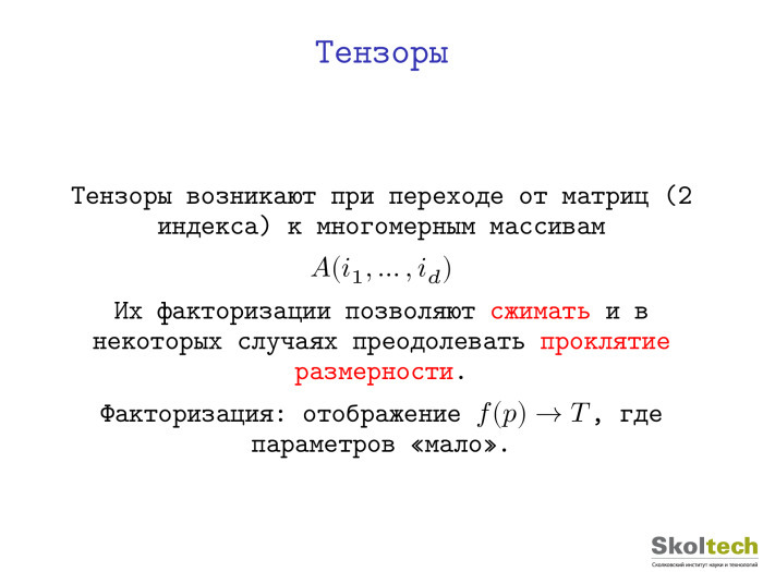
And what will happen if, instead of A (i, j), we write A (i, jk), and also try to separate the variables. Hence, the problem of tensor expansions arises in a completely natural way. We have a tensor - I understand a multidimensional array, a simple two-dimensional table as a tensor - and we want to compress these multidimensional arrays roughly, to construct a low-parametric representation and, usually beautiful words say, to overcome the curse of dimension. In fact, this term - he, as always, appeared in a completely different context with a completely different task, in the work of Bellman in 1961. But now it is used in the sense that n to the power of d is very bad. If you want to increase d, then you will have an exponential growth, etc.
Factorization in the most general sense: you are trying to choose a certain class of tensors, which arises in your applied task, and to construct such a little-parametric representation, that using it you can quickly enough recover the tensor itself. And there are few parameters. In principle, we can say that neural networks in some sense solve the problem of approximating tensors, because they are trying to build a mapping from the parameter space somewhere else.

If in factorization problems, that is, in representations in the form of a product of simple objects, there are matrices and products of matrices with tensors, then determining tensors is a more difficult task. But if we look at the index record of the incomplete singular decomposition of a low-ranking approximation, a similar formula will arise in a completely natural way. Here she is. We are trying to approximate the tensor by objects that are products of a function of one discrete variable, the function t1 is multiplied by the function t2. The idea is completely natural. If the term is only one, you will not bring anything closer. And if you allow to take a fairly small number of parameters, a very interesting class of tensors arises, which is used explicitly or implicitly in many problems of the methods. We can say that approximately this format is used in quantum chemistry to represent the wave function. There is also antisymmetry, instead of a work a determinant arises - but a whole huge field of science is based, in fact, on such a separable approximation.
Therefore, it is naturally interesting to study the properties, to understand what is happening here, and so on.

This entity — the representation as the sum of the product of functions of one variable — is called the canonical decomposition. It was first proposed around 1927. Then it was used far from mathematics. There were jobs in statistics, in journals — such as Chemometrics, Psychomatrix — where people got data cubes. There are signs - something happened. Thus, they built multifactor models. These matrixes of factors can be interpreted as certain factors. From them, in turn, it is possible to draw any conclusions.
If we count the number of parameters, we get dnr parameters. If r is small, then everything is fine. But the problem that I am trying to solve is that, in principle, to calculate such an approximation, even if it is known that it exists, is a difficult task. One can even say that it is NP-complex in the general case, just like the task of computing the rank. For the matrix it is not. You can calculate the rank of the matrix - for example, with the help of Gaussian exceptions, this can be done in a polynomial number of operations. This is not the case.
There is an example of a 9x9x9 tensor, for which the exact value of the minimum number of terms is still unknown. It is known that it is not more than 23 and not less than 21. Supercomputers, simple polynomial: it is a matter of solvability of a system of polynomial equations. But such a task can be very difficult. A tensor is of practical importance. The rank of this tensor is related to the complexity index of the matrix multiplication algorithm. The Strassen-logarithm is binary from seven. Accordingly, in fact, the problem of calculating the exponential reduces to calculating the canonical rank of a certain tensor.
In many applications, this view for some particular tensor works well. But in general this task is bad.
Recently, the work of quite respected people appeared, where they try to connect this representation with dividing variables with deep neural networks and prove some results. In fact, if they are deciphered, they are quite interesting algebraic results on tensor decompositions. If we translate the results into the language of tensor expansions, it turns out that one tensor decomposition, the canonical one, is better than the other. The one that is better, I have not shown, but the canonical has shown. The canonical is bad in that sense. This conclusion is justified by the fact that the canonical architecture is shallow, not deep, but it must be deep, more extensive, and so on.
So let's try to go smoothly to this. For canonical decomposition, optimization algorithms converge slowly, that is, there is a swamp, etc. If you look at this formula, everyone who is familiar with linear algebra will immediately understand which algorithm can be used. You can use gradient descents - fix all factors except one and get a linear least squares problem. But this method will be quite slow.
Such a model has one good property: if a solution is found after all, it is unique up to trivial things. For example, matrix decomposition problems do not arise when you can insert s, s-1. If canonical decomposition is counted, it is unique, and that is good. But unfortunately, it is sometimes quite difficult to count it.

There is another Tucker decomposition. It was some kind of psychometric. The idea is to introduce a gluing factor here, so that everyone does not have a connection with each. Everything is good, this decomposition becomes stable, the best approximation always exists. But if you try to use it, say, for d = 10, then an auxiliary two-dimensional array will appear that needs to be stored, and the curse of the dimension, although in a weakened form, will remain.
Yes, for example, for three-dimensional and four-dimensional problems, the Tacker decomposition works fine. There is a fairly large number of works where it applies. But nevertheless, our ultimate goal is not this.

We want to get something where, by default, there is no exponential number of parameters, but where we can count everything. The initial idea was quite simple: if everything is good for matrices, let's make matrices from tensors, multidimensional arrays. How to do it? Simple enough. We have d indices - let's divide them into groups, make matrices, count expansions.
We break. We declare one part of the indices as string indices, the other part as column indices. Maybe somehow rearranged. In MATLAB and Python, this is all done with the reshape and transpose command, we assume low-rank approximation. Another question is how we do it.
Naturally, we can try to make the resulting small arrays recursively. It is easy enough to see that if we make them naively, we will have something like this: r log d . It is no longer exponential, but r will be sufficiently large.
If you do this carefully, then - I will say only one phrase - there will be one additional index. It should be considered a new index. Suppose we had a nine-dimensional array and we divided the indices into 5 + 4, decomposed, obtained one additional index, obtained one six-dimensional and one five-dimensional tensor and continue to decompose them. In this form, no exponential complexity arises, and a representation is obtained that has this number of parameters. And if someone told us that all the resulting matrices have a small rank? Such recursive structure turns out. It is quite nasty, programming it is quite nasty, I was too lazy to do it.

At some point, I realized that you can choose the simplest form of this structure - which, nevertheless, is quite powerful. This is what became the tensor train, the tensor-train. We have proposed this, the name stuck. Then it turned out that we were, of course, not the first to invent it. In solid state physics, it was known as matrix product states. But I repeat on every report that a good thing must be opened at least twice - otherwise it is not very clear if it is good. At least, this view was opened at least two, or even two and a half times, or even three.
Here is a presentation, the decomposition and study of which I have been doing for the last six or seven years, and I can’t fully say that it has been studied.
We represent the tensor as a product of objects that depend on only one index. In fact, we are talking about the separation of variables, but with one small exception: now these little things are matrices. We multiply to get the values of the tensors of a point, these matrices. The first element is a line, then a matrix, a matrix, a column — we get a number. And these matrices depend on the parameters, they can be stored as a three-dimensional tensor. We have a collection of matrices, at the beginning - a collection of lines. We say: we need a zero line from here, a fifth matrix from here, a third one from here — we simply multiply them. It is clear that the calculation of the element takes dr 2 operations. In the index view too. Compact this kind.
It seems that nothing changes much, but in fact such a representation retains all the properties of singular decomposition. It can be calculated, it can be orthogonalized, it is possible to find the best approximations. This is a non-parametric manifold in the set of all tensors, but we can say that we - if we are lucky and have a solution on it - we will easily find it.

Here are some properties. We now have more than one rank. There is only one rank in the matrix, column or lower case, but they are the same for the matrix, so lucky. For tensors, ranks are many. The number r at the beginning is the canonical rank. Here we have the rank d-1. For each d is your rank, we have many ranks. Nevertheless, all these complexity-defining ranks and memory for storing such a representation can be counted, at least theoretically, as the ranks of some matrices, the so-called reamers. We take a multidimensional array, turn it into matrices, count ranks - aha, there is a decomposition with such ranks.
Why is it called format? If our objects are stored in this format, algebraic operations of addition, multiplication, norm calculations can be done directly - without leaving the format. At the same time, something happens anyway. For example, if we add two tensors, the result will have a rank that does not exceed the sum of the ranks. If you do this many times in any iterative process, then the rank will become very large - even though the dependence on d is linear, and r is quadratic. You can work calmly with rank 100-200. Physicists on clusters can work with 4000-5000 ranks, but they can no longer, because it is necessary to store rather large dense matrices.
But there is a very simple and beautiful algebraic algorithm that allows decreasing ranks. I have some allowable accuracy in the Frabenius norm and I want to find the minimum ranks that give accuracy. But I simultaneously reduce the ranks. Rounding When you work with floating point numbers, you do not store all 100 digits. You leave only 16 digits. We find those parameters, such a size of these matrices, which give an acceptable accuracy. There is a robust robust algorithm that does this — it takes 20–30 lines in MATLAB or in Python.
There is one more beautiful thing. Physicists did not know her exactly. I am proud of this result, he is mine with my then chief, Yevgeny Evgenievich Tartyshnikov. If we know that the tensor given to us has such a structure, then we can definitely restore it by dnr 2 elements. That is, without calculating all the elements, we can look at a small number of them and restore the entire tensor, without using any bases, nothing. This is an interesting fact, it is not for matrices how well-known it could be. There is d = 2, the matrix of rank r. It can be restored by r columns and r rows.
When we have such a variety, we can minimize the functional with a restriction on the ranks. Standard situation: we don’t have access to the elements, but there is some quality functionality that we would like to minimize. For this, a whole separate direction of research of the question arises, how to optimize with the indicated limitations. This is not a convex set, but it has many interesting topological properties that require separate study.
Recently, mainly for problems arising from a partial differential equation, it is finally possible to prove the estimate that ranks behave logarithmically depending on the required accuracy. There are whole classes of problems where such representations are quasioptimal.

Let's run through how to count TT-ranks. We take the matrix, the first k indices are considered lowercase indices, the last dk - columnar. , . .
. , . . — d-1 , . , 10-6, .
d . — . , . 1010, 100100. , 1000010000, .

dnr 3 . , - .
. - 100 , 10 , .
. .

. , . . , , . . , .
r, r r , . , , , .
, , . , , . — , 5, 5 5 , .
, . , .
, , , . - . , . , , . . : , .
. , -, . , . , , . . , .
, , .
— , . , d-. d- , . . 2 d 2222. , . . , , , .
— , - , — , - .
. . , . , , , . — .
: ttpy Python TT-Toolbox MATLAB. , , , , . , , .
. , , , . , , - , . - . , : . 10 -6 10 -8 . — , — . — , . , , , . , , , - . We'll see.
, - , . TensorFlow . , — , . - , . , , .
, . . 2 60 . . , n 3 , n = 2 d , 220, . 2222, 60- . .
, : 2 d, 60, , 50. , .
, . , , , , . .

, . TensorNet, , NIPS . , . , , .
. . , .
, . , , . , . , , : , .
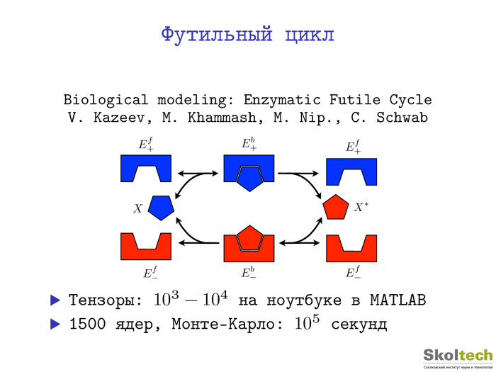
. : , , , , . , , . , . , — , . , . , , . -, . 1500 — 10 5 . MATLAB . .

. 12 , 12- , 30 12 . .

Exponential Machines, x1, x2, , 2 d . 2222 : . Works. , , .
. , , . , - — , . RecSys. Polara. , , . : . : , « », SVD « ». « » . . : « — » « — — » , . - . , , , - : , , , . , .

, — . . , deep learning. , arithmetic circuit. , .
, GitHub , . , .
Under the cut - the decoding and most of the slides.
There is a small - relatively machine learning - community that deals with linear algebra. There is linear algebra, and there are people in it who are engaged in multilinear algebra, tensor decompositions. I treat them. A sufficiently large number of interesting results were obtained there, but due to the ability of the community to self-organize and not go outside, some of these results are unknown. By the way, this also applies to linear algebra. If you look at the articles of the leading conferences of the NIPS, ICML, etc., then you can see quite a lot of articles related to the trivial facts of linear algebra. This happens, but nonetheless.
')
We will talk about tensor expansions, but first we must say about matrix expansions.
Matrices. Just a two-dimensional table. The matrix decomposition is a representation of the matrix in the form of products of Boolean primes. In fact, they are used everywhere, everyone has mobile phones, and while you are sitting, they solve linear systems, transfer data, decompose matrices. True, these matrices are very small - 4x4, 8x8. But in practice, these matrices are very important.
I must say that there is a LU decomposition, Gauss decomposition, QR decomposition, but I will mainly talk about singular decomposition, which for some reason, for example, in linear algebra courses in our universities is undeservedly forgotten. They read such nonsense from the point of view of computational science, like the Jordan form, which is not used anywhere. Singular decomposition is usually somewhere at the end, optional, etc. This is wrong. If we take the book by Golub and van Louna , “Matrix Computations,” then it starts with neither LU- nor QR-, but with singular decomposition. This representation of the matrix as a product of the unitary, diagonal, and unitary.
It is good about matrix expansions that there really is a lot of information about them. For basic expansions, there are effective algorithms, they are robust, there is software that you can call in MATLAB, in Python, they are written in Fortran. Correctly regard this as a single operation that can be counted, and you are sure that you will get an accurate result - that you do not need to do any gradient descents. Actually it is one quantum of operation. If you reduced your task to calculating matrix expansions, then you actually solved it. This, for example, underlies the various spectral methods. For example, if there is an EM algorithm, it is iterative, it has a slow convergence. And if you managed to get the spectral method, then you are great and you will have a solution in one step.
Directly the same singular expansion does not solve any problem, but is a sort of building block for solving common problems. Let's go back to mobile phones. This example bothers me for obvious reasons: we work with telecommunication companies that really need it.
There is a look at what a singular decomposition is and write it in index form, we get the following formula. This leads to the classic old idea - to the separation of variables, if we return to the first courses of the university. We decompose x from t, and here we separate I from j, one discrete index is separated from another, that is, we represent a function of two variables as a product of functions from one variable. It is clear that almost no function in this form is approaching, but if you write the sum of such functions, you will get a fairly wide class.
In fact, the main application of the singular value decomposition is the construction of such low-rank approximations. This is a matrix of rank r, and, naturally, we are interested in the case when the rank is substantially less than the total size of the matrix.
Everything is good here. We can fix the rank, set the task of finding the best approximation and the solution will be given for the singular decomposition. In fact, much more is known there and it can be done faster than with the help of singular decomposition: without calculating all the elements of the matrix, etc. There is a big beautiful theory - the theory of low-rank matrices, which continues to evolve and is far from being closed.
Nevertheless, it is not closed, but I want to do more than two indices.
My initial interest in this topic was purely theoretical. We know how to do something with matrices, decompose them, to represent them in some applications - it does not matter in which ones yet. At the end I will say.
And what will happen if, instead of A (i, j), we write A (i, jk), and also try to separate the variables. Hence, the problem of tensor expansions arises in a completely natural way. We have a tensor - I understand a multidimensional array, a simple two-dimensional table as a tensor - and we want to compress these multidimensional arrays roughly, to construct a low-parametric representation and, usually beautiful words say, to overcome the curse of dimension. In fact, this term - he, as always, appeared in a completely different context with a completely different task, in the work of Bellman in 1961. But now it is used in the sense that n to the power of d is very bad. If you want to increase d, then you will have an exponential growth, etc.
Factorization in the most general sense: you are trying to choose a certain class of tensors, which arises in your applied task, and to construct such a little-parametric representation, that using it you can quickly enough recover the tensor itself. And there are few parameters. In principle, we can say that neural networks in some sense solve the problem of approximating tensors, because they are trying to build a mapping from the parameter space somewhere else.
If in factorization problems, that is, in representations in the form of a product of simple objects, there are matrices and products of matrices with tensors, then determining tensors is a more difficult task. But if we look at the index record of the incomplete singular decomposition of a low-ranking approximation, a similar formula will arise in a completely natural way. Here she is. We are trying to approximate the tensor by objects that are products of a function of one discrete variable, the function t1 is multiplied by the function t2. The idea is completely natural. If the term is only one, you will not bring anything closer. And if you allow to take a fairly small number of parameters, a very interesting class of tensors arises, which is used explicitly or implicitly in many problems of the methods. We can say that approximately this format is used in quantum chemistry to represent the wave function. There is also antisymmetry, instead of a work a determinant arises - but a whole huge field of science is based, in fact, on such a separable approximation.
Therefore, it is naturally interesting to study the properties, to understand what is happening here, and so on.
This entity — the representation as the sum of the product of functions of one variable — is called the canonical decomposition. It was first proposed around 1927. Then it was used far from mathematics. There were jobs in statistics, in journals — such as Chemometrics, Psychomatrix — where people got data cubes. There are signs - something happened. Thus, they built multifactor models. These matrixes of factors can be interpreted as certain factors. From them, in turn, it is possible to draw any conclusions.
If we count the number of parameters, we get dnr parameters. If r is small, then everything is fine. But the problem that I am trying to solve is that, in principle, to calculate such an approximation, even if it is known that it exists, is a difficult task. One can even say that it is NP-complex in the general case, just like the task of computing the rank. For the matrix it is not. You can calculate the rank of the matrix - for example, with the help of Gaussian exceptions, this can be done in a polynomial number of operations. This is not the case.
There is an example of a 9x9x9 tensor, for which the exact value of the minimum number of terms is still unknown. It is known that it is not more than 23 and not less than 21. Supercomputers, simple polynomial: it is a matter of solvability of a system of polynomial equations. But such a task can be very difficult. A tensor is of practical importance. The rank of this tensor is related to the complexity index of the matrix multiplication algorithm. The Strassen-logarithm is binary from seven. Accordingly, in fact, the problem of calculating the exponential reduces to calculating the canonical rank of a certain tensor.
In many applications, this view for some particular tensor works well. But in general this task is bad.
Recently, the work of quite respected people appeared, where they try to connect this representation with dividing variables with deep neural networks and prove some results. In fact, if they are deciphered, they are quite interesting algebraic results on tensor decompositions. If we translate the results into the language of tensor expansions, it turns out that one tensor decomposition, the canonical one, is better than the other. The one that is better, I have not shown, but the canonical has shown. The canonical is bad in that sense. This conclusion is justified by the fact that the canonical architecture is shallow, not deep, but it must be deep, more extensive, and so on.
So let's try to go smoothly to this. For canonical decomposition, optimization algorithms converge slowly, that is, there is a swamp, etc. If you look at this formula, everyone who is familiar with linear algebra will immediately understand which algorithm can be used. You can use gradient descents - fix all factors except one and get a linear least squares problem. But this method will be quite slow.
Such a model has one good property: if a solution is found after all, it is unique up to trivial things. For example, matrix decomposition problems do not arise when you can insert s, s-1. If canonical decomposition is counted, it is unique, and that is good. But unfortunately, it is sometimes quite difficult to count it.
There is another Tucker decomposition. It was some kind of psychometric. The idea is to introduce a gluing factor here, so that everyone does not have a connection with each. Everything is good, this decomposition becomes stable, the best approximation always exists. But if you try to use it, say, for d = 10, then an auxiliary two-dimensional array will appear that needs to be stored, and the curse of the dimension, although in a weakened form, will remain.
Yes, for example, for three-dimensional and four-dimensional problems, the Tacker decomposition works fine. There is a fairly large number of works where it applies. But nevertheless, our ultimate goal is not this.
We want to get something where, by default, there is no exponential number of parameters, but where we can count everything. The initial idea was quite simple: if everything is good for matrices, let's make matrices from tensors, multidimensional arrays. How to do it? Simple enough. We have d indices - let's divide them into groups, make matrices, count expansions.
We break. We declare one part of the indices as string indices, the other part as column indices. Maybe somehow rearranged. In MATLAB and Python, this is all done with the reshape and transpose command, we assume low-rank approximation. Another question is how we do it.
Naturally, we can try to make the resulting small arrays recursively. It is easy enough to see that if we make them naively, we will have something like this: r log d . It is no longer exponential, but r will be sufficiently large.
If you do this carefully, then - I will say only one phrase - there will be one additional index. It should be considered a new index. Suppose we had a nine-dimensional array and we divided the indices into 5 + 4, decomposed, obtained one additional index, obtained one six-dimensional and one five-dimensional tensor and continue to decompose them. In this form, no exponential complexity arises, and a representation is obtained that has this number of parameters. And if someone told us that all the resulting matrices have a small rank? Such recursive structure turns out. It is quite nasty, programming it is quite nasty, I was too lazy to do it.
At some point, I realized that you can choose the simplest form of this structure - which, nevertheless, is quite powerful. This is what became the tensor train, the tensor-train. We have proposed this, the name stuck. Then it turned out that we were, of course, not the first to invent it. In solid state physics, it was known as matrix product states. But I repeat on every report that a good thing must be opened at least twice - otherwise it is not very clear if it is good. At least, this view was opened at least two, or even two and a half times, or even three.
Here is a presentation, the decomposition and study of which I have been doing for the last six or seven years, and I can’t fully say that it has been studied.
We represent the tensor as a product of objects that depend on only one index. In fact, we are talking about the separation of variables, but with one small exception: now these little things are matrices. We multiply to get the values of the tensors of a point, these matrices. The first element is a line, then a matrix, a matrix, a column — we get a number. And these matrices depend on the parameters, they can be stored as a three-dimensional tensor. We have a collection of matrices, at the beginning - a collection of lines. We say: we need a zero line from here, a fifth matrix from here, a third one from here — we simply multiply them. It is clear that the calculation of the element takes dr 2 operations. In the index view too. Compact this kind.
It seems that nothing changes much, but in fact such a representation retains all the properties of singular decomposition. It can be calculated, it can be orthogonalized, it is possible to find the best approximations. This is a non-parametric manifold in the set of all tensors, but we can say that we - if we are lucky and have a solution on it - we will easily find it.
Here are some properties. We now have more than one rank. There is only one rank in the matrix, column or lower case, but they are the same for the matrix, so lucky. For tensors, ranks are many. The number r at the beginning is the canonical rank. Here we have the rank d-1. For each d is your rank, we have many ranks. Nevertheless, all these complexity-defining ranks and memory for storing such a representation can be counted, at least theoretically, as the ranks of some matrices, the so-called reamers. We take a multidimensional array, turn it into matrices, count ranks - aha, there is a decomposition with such ranks.
Why is it called format? If our objects are stored in this format, algebraic operations of addition, multiplication, norm calculations can be done directly - without leaving the format. At the same time, something happens anyway. For example, if we add two tensors, the result will have a rank that does not exceed the sum of the ranks. If you do this many times in any iterative process, then the rank will become very large - even though the dependence on d is linear, and r is quadratic. You can work calmly with rank 100-200. Physicists on clusters can work with 4000-5000 ranks, but they can no longer, because it is necessary to store rather large dense matrices.
But there is a very simple and beautiful algebraic algorithm that allows decreasing ranks. I have some allowable accuracy in the Frabenius norm and I want to find the minimum ranks that give accuracy. But I simultaneously reduce the ranks. Rounding When you work with floating point numbers, you do not store all 100 digits. You leave only 16 digits. We find those parameters, such a size of these matrices, which give an acceptable accuracy. There is a robust robust algorithm that does this — it takes 20–30 lines in MATLAB or in Python.
There is one more beautiful thing. Physicists did not know her exactly. I am proud of this result, he is mine with my then chief, Yevgeny Evgenievich Tartyshnikov. If we know that the tensor given to us has such a structure, then we can definitely restore it by dnr 2 elements. That is, without calculating all the elements, we can look at a small number of them and restore the entire tensor, without using any bases, nothing. This is an interesting fact, it is not for matrices how well-known it could be. There is d = 2, the matrix of rank r. It can be restored by r columns and r rows.
When we have such a variety, we can minimize the functional with a restriction on the ranks. Standard situation: we don’t have access to the elements, but there is some quality functionality that we would like to minimize. For this, a whole separate direction of research of the question arises, how to optimize with the indicated limitations. This is not a convex set, but it has many interesting topological properties that require separate study.
Recently, mainly for problems arising from a partial differential equation, it is finally possible to prove the estimate that ranks behave logarithmically depending on the required accuracy. There are whole classes of problems where such representations are quasioptimal.
Let's run through how to count TT-ranks. We take the matrix, the first k indices are considered lowercase indices, the last dk - columnar. , . .
. , . . — d-1 , . , 10-6, .
d . — . , . 1010, 100100. , 1000010000, .
dnr 3 . , - .
. - 100 , 10 , .
. .
. , . . , , . . , .
r, r r , . , , , .
, , . , , . — , 5, 5 5 , .
, . , .
, , , . - . , . , , . . : , .
. , -, . , . , , . . , .
, , .
— , . , d-. d- , . . 2 d 2222. , . . , , , .
— , - , — , - .
. . , . , , , . — .
: ttpy Python TT-Toolbox MATLAB. , , , , . , , .
. , , , . , , - , . - . , : . 10 -6 10 -8 . — , — . — , . , , , . , , , - . We'll see.
, - , . TensorFlow . , — , . - , . , , .
, . . 2 60 . . , n 3 , n = 2 d , 220, . 2222, 60- . .
, : 2 d, 60, , 50. , .
, . , , , , . .
, . TensorNet, , NIPS . , . , , .
. . , .
, . , , . , . , , : , .
. : , , , , . , , . , . , — , . , . , , . -, . 1500 — 10 5 . MATLAB . .
. 12 , 12- , 30 12 . .
Exponential Machines, x1, x2, , 2 d . 2222 : . Works. , , .
. , , . , - — , . RecSys. Polara. , , . : . : , « », SVD « ». « » . . : « — » « — — » , . - . , , , - : , , , . , .
, — . . , deep learning. , arithmetic circuit. , .
, GitHub , . , .
Source: https://habr.com/ru/post/313892/
All Articles