[Bookmark] Zoo neural network architectures. Part 1

This is the first part, here is the second.
It is not easy to keep track of all the neural network architectures that continually arise lately. Even understanding all the abbreviations that professionals throw at first may seem like an impossible task.

Therefore, I decided to make a cheat sheet for such architectures. Most of them are neural networks, but some are animals of a different breed. Although all these architectures are presented as new and unique, when I portrayed their structure, internal communications have become much clearer.

')


The image of neural networks in the form of graphs has one drawback: the graph will not show how the network works. For example, a variational autoencoder (variational autoencoders, VAE) looks exactly like a simple autoencoder (AE), while the learning process of these neural networks is completely different. Usage scenarios differ even more: in VAE, noise comes in from the input from which they receive a new vector, while AE simply finds the closest corresponding vector to the input data from those that they “remember”. I will also add that this review has no purpose to explain the work of each of the topologies from the inside (but this will be the topic of one of the following articles).

It should be noted that not all (although most) of the abbreviations used here are generally accepted. RNN is sometimes understood as recursive neural networks, but usually this abbreviation means recurrent neural network. But that's not all: in many sources you will find RNN as a designation for any recurrent architecture, including LSTM, GRU, and even bidirectional options. Sometimes a similar confusion occurs with AE: VAE, DAE and the like can simply be called AE. Many abbreviations contain different amounts of N at the end: one can say “convolutional neural network” - CNN (Convolutional Neural Network), or just “convolutional network” - CN.

It is almost impossible to compile a complete list of topologies, since new ones appear constantly. Even if you specifically look for publications, it can be difficult to find them, and some can simply be overlooked. Therefore, although this list will help you create an idea of ​​the world of artificial intelligence, please do not consider it exhaustive, especially if you read the article long after its appearance.

For each of the architectures shown in the diagram, I gave a very short description. Some of them will be useful if you are familiar with several architectures, but are not specifically familiar with this one.

---

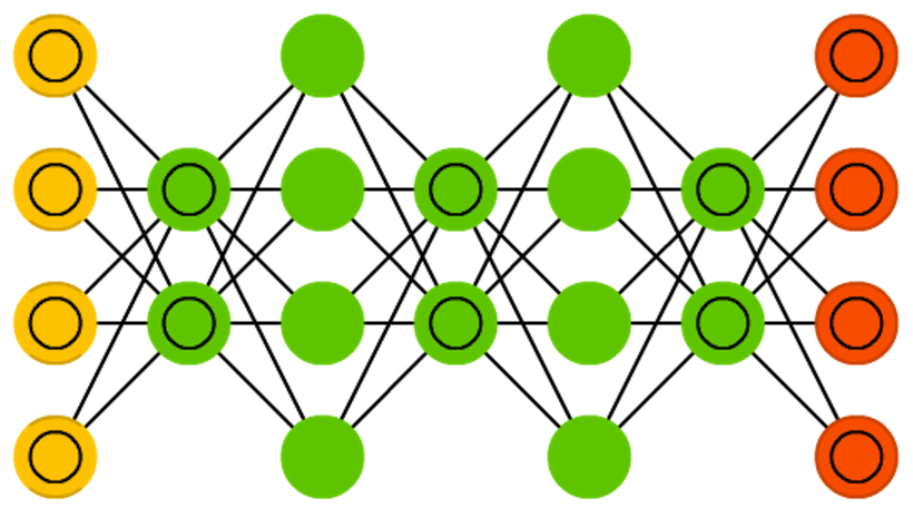
Forward distribution networks (Feed forward neural networks, FF or FFNN) and perceptrons (Perceptrons, P) are very simple - they transfer information from input to output. It is believed that neural networks have layers, each of which consists of input, hidden or output neurons. Neurons of one layer are not connected with each other, with each neuron of this layer associated with each neuron of the adjacent layer. The simplest working network consists of two input and one output neuron and can simulate a logic gate - the basic element of a digital circuit that performs an elementary logic operation. FFNN is usually trained in the back-propagation method of error, feeding models to the input of a pair of input and expected output data. The error is usually understood to mean different degrees of deviation of the output from the original (for example, the standard deviation or the sum of the moduli of differences). Provided that the network has a sufficient number of hidden neurons, in theory it will always be able to establish a connection between the input and output data. In practice, the use of direct distribution networks is limited, and more often they are shared with other networks.

Rosenblatt, Frank. “The perceptron: a probabilistic model for information storage in the brain.” Psychological review 65.6 (1958): 386.

» Original Paper PDF

---

Radial basis functions (RBF) networks are FFNN with a radial basis function as an activation function. There is nothing more to add. We do not want to say that it is not used, but most FFNN with other activation functions are usually not allocated to separate groups.

Broomhead, David S., and David Lowe. Radial basis functions, multi-variable functional interpolation and adaptive networks. No. RSRE-MEMO-4148. ROYAL SIGNALS AND RADAR ESTABLISHMENT MALVERN (UNITED KINGDOM), 1988.

» Original Paper PDF

---

The Hopfield neural network is a fully connected network (each neuron is connected to each), where each neuron appears in all three forms. Each neuron serves as an input to learning, hidden during it and a weekend after. The weights matrix is ​​selected so that all the “memorized” vectors would be proper for it. Once a system is trained in one or more images, it will converge to one of its known images, because only one of these states is stationary. Note that this does not necessarily correspond to the desired state (unfortunately, we do not have a magic black box). The system is only partially stabilized due to the fact that the total “energy” or “temperature” of the network gradually decreases during training. Each neuron has an activation threshold commensurate with this temperature, and if the sum of the input data exceeds this threshold, the neuron can go into one of two states (usually -1 or 1, sometimes 0 or 1). Network nodes can be updated in parallel, but most often it happens sequentially. In the latter case, a random sequence is generated, which determines the order in which the neurons will update their state. When each of the neurons is updated and their state no longer changes, the network comes to a stationary state. Such networks are often called associative memory, since they converge with the state closest to the given one: as a person, seeing half of the picture, can finish drawing the missing half, so the neural network, receiving a half-noisy picture at the entrance, completes it to the whole.

Hopfield, John J. “Emergency collective computational abilities and systems”. ”79.8 (1982): 2554-2558.

» Original Paper PDF

---

Markov Chains (Markov Chains, MC or discrete time Markov Chain, DTMC) are a kind of predecessor of Boltzmann machines (BM) and Hopfield networks (HN). In Markov chains, we set the transition probabilities from the current state to the neighboring ones. In addition, this chain has no memory: the subsequent state depends only on the current one and does not depend on all past states. Although the Markov chain cannot be called a neural network, it is close to them and forms the theoretical basis for BM and HN. Markov chains are also not always fully connected.

Hayes, Brian. “First links in the Markov chain.” American Scientist 101.2 (2013): 252.

» Original Paper PDF

---

Boltzmann machines (BM) machines are in many ways similar to the Hopfield network, but in them some neurons are marked as input and some remain hidden. Input neurons become output when all neurons on the network update their states. First, weights are assigned randomly, then learning is done using the method of back propagation, or more recently, using the contrastive divergence algorithm (when the gradient is calculated using a Markov chain). BM is a stochastic neural network, since the Markov chain is involved in the training. The process of learning and working here is almost the same as in the Hopfield network: certain initial states are assigned to neurons, and then the chain begins to function freely. In the process of work, neurons can assume any state, and we constantly move between input and hidden neurons. Activation is governed by the value of the total temperature, with a decrease in which the energy of neurons is reduced. Reducing energy causes stabilization of neurons. Thus, if the temperature is set correctly, the system reaches an equilibrium.

Hinton, Geoffrey E., and Terrence J. Sejnowski. “Learning and releasing in Boltzmann machines.” Parallel distributed processing: Exploration in the microstructure of cognition 1 (1986): 282-317.

» Original Paper PDF

---

The limited Boltzmann machine (Restricted Boltzmann machine, RBM) is , surprisingly, very similar to the normal Boltzmann machine. The main difference between RBM and BM is that they are limited and therefore more convenient to use. In them, each neuron is not connected with each, but only each group of neurons is connected to other groups. Input neurons are not connected to each other, there are no connections and between hidden neurons. RBM can be trained in the same way as FFPN, with a small difference: instead of transferring data forward and subsequent back propagation of error, data is transmitted back and forth (to the first layer), and then forward and backward propagation is applied .

Smolensky, Paul. Information processing in dynamical systems: Foundations of harmony theory. No. CU-CS-321-86. COLORADO UNIV AT BOULDER DEPT OF COMPUTER SCIENCE, 1986.

» Original Paper PDF

---

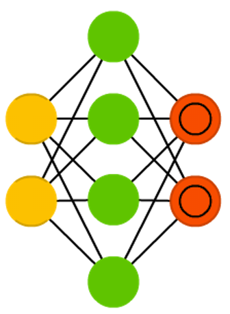
Autoencoders (AE) - something like FFNN, this is rather a different way to use FFNN than a fundamentally new architecture. The main idea of ​​avtoenkoderov - automatic encoding (as when compressing, and not when encrypting) information, hence the name. The network resembles an hourglass shape, since the hidden layer is smaller than the input and output; moreover, it is symmetric with respect to the middle layers (one or two, depending on the parity / oddness of the total number of layers). The smallest layer is almost always the middle one, information is maximally compressed in it. All that is located to the middle - the coding part, above the middle - decoding, and in the middle (you will not believe) - the code. AE is trained in the back propagation method of an error, giving input data and setting an error equal to the difference between input and output. AE can be constructed symmetric and in terms of weights, exposing the encoding weights equal decoding.

Bourlard, Hervé, and Yves Kamp. “Auto-association by multilayer perceptrons and singular value decomposition.” Biological cybernetics 59.4-5 (1988): 291-294.

» Original Paper PDF

---

A sparse autoencoder (Sparse autoencoder, AE) is to some extent an antipode of AE. Instead of teaching the network to represent blocks of information in a smaller “space,” we encode information so that it takes up more space. And instead of forcing the system to converge in the center, and then expand back to its original size, we, on the contrary, increase the middle layers. Networks of this type can be used to extract many small details from a data set. If we began to teach SAE in the same way as AE, we would get in most cases an absolutely useless network, where the output is exactly the same as at the input. To avoid this, instead of the input data, we output the input data plus a penalty for the number of activated neurons in the hidden layer. To a certain extent, this resembles a biological neural network (spiking neural network), in which not all neurons are constantly in an excited state.

Marc'Aurelio Ranzato, Christopher Poultney, Sumit Chopra, and Yann LeCun. “Efficient learning of an energy-based model.” Proceedings of NIPS. 2007

» Original Paper PDF

---

The architecture of variational autoencoders (VAE) is the same as that of ordinary, but they are taught another - the approximate probability distribution of input samples. This is to some extent a return to basics, as the VAE is a little closer to the Boltzmann machines. However, they rely on Bayesian mathematics regarding probabilistic judgments and independence, which are intuitive but require complex calculations. The basic principle can be formulated as follows: take into account the degree of influence of one event on another. If a certain event occurs in one place, and another event happens somewhere else, then these events are not necessarily related. If they are not related, then the propagation of the error should take this into account. This is a useful approach, since neural networks are a kind of huge graphs, and sometimes it is useful to exclude the influence of some neurons on others, falling into the lower layers.

Kingma, Diederik P., and Max Welling. “Auto-encoding variational bayes.” ArXiv preprint arXiv: 1312.6114 (2013).

» Original Paper PDF

---

Noise-canceling (noise-resistant) auto-encoders (Denoising autoencoders, DAE) - this is AE, which we do not just input data to the input, but noise data (for example, making the picture more grainy). Nevertheless, we calculate the error by the former method, comparing the output sample with the original without noise. Thus, the network does not memorize small details, but large features, since memorizing small details that are constantly changing due to noise often leads nowhere.

Vincent, Pascal, et al. “Extracting and composing robust features with denoising autoencoders.” Proceedings of the 25th international conference on Machine Learning. ACM, 2008.

» Original Paper PDF

---

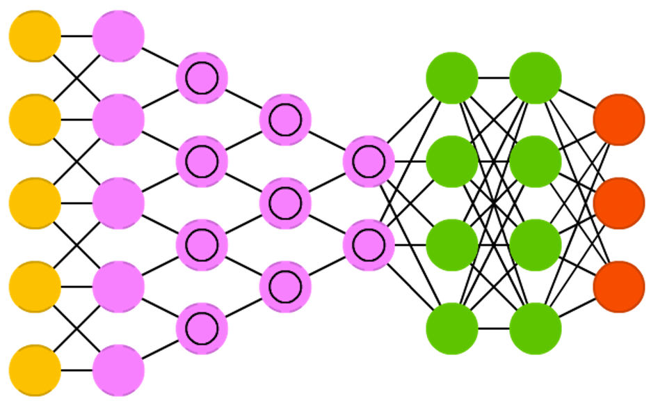
Deep trust networks (Deep belief networks, DBN) are networks composed of several RBM or VAE. Such networks proved to be effectively trained one after another, when each network must learn to code the previous one. This method is also called “greedy learning”, it is to make the best decision at the moment to get a suitable, but perhaps not the optimal result. DBNs can be trained by contrastive divergence or backpropagation and learn to present data as a probabilistic model, exactly like RBM or VAE. Once a trained and stationary model can be used to generate new data.

Bengio, Yoshua, et al. “Greedy layer-wise training of deep networks.” Advances in neural information processing systems 19 (2007): 153.

» Original Paper PDF

---

Convolutional neural networks (convolutional neural networks, CNN) and deep convolutional neural networks (deep convolutional neural networks, DCNN) are radically different from other networks. They are mainly used for image processing, sometimes for audio and other types of input data. A typical way of using CNN is image classification: if a cat image is input, the network will produce a cat, if the dog’s picture is a dog. Such networks typically use a “scanner” that does not process all data at one time. For example, if you have an image of 200x200, you want to build a network layer of 40 thousand nodes. Instead, the network counts a 20x20 square (usually from the upper left corner), then moves 1 pixel and counts a new square, and so on. Notice that we do not break the image into squares, but rather we crawl on it. These inputs are then transmitted through convolutional layers, in which not all nodes are interconnected. Instead, each node is connected only to its closest neighbors. These layers tend to shrink with depth, and usually they are reduced by one of the dividers of the amount of input data (for example, 20 nodes in the next layer will turn into 10, in the next one - in 5), powers of two are often used. In addition to convolutional layers, there are also so-called pooling layers. Combining is a way to reduce the dimension of the data received, for example, the most red pixel is selected and transmitted from a 2x2 square. In practice, by the end of CNN attach FFNN for further data processing. Such networks are called deep (DCNN), but their names are usually interchangeable.

LeCun, Yann, et al. “Gradient-based learning to document recognition.” Proceedings of the IEEE 86.11 (1998): 2278-2324.

» Original Paper PDF

---

Deploying neural networks (deconvolutional networks, DN) , also called reverse graphical networks, are converse neural networks in reverse. Imagine that you transmit the word “cat” to the network and train it to generate pictures of cats by comparing the resulting pictures with real images of cats. DNN can also be combined with FFNN. It should be noted that in most cases the network does not transmit a string, but a binary classifying vector: for example, <0, 1> is a cat, <1, 0> is a dog, and <1, 1> is both a cat and a dog. Instead of combining layers, which are often found in CNN, there are similar inverse operations, usually interpolation or extrapolation.

Zeiler, Matthew D., et al. “Deconvolutional networks.” Computer Vision and Pattern Recognition (CVPR), 2010 IEEE Conference on. IEEE, 2010.

» Original Paper PDF

---

Read the sequel.

Oh, and come to work with us? :)

wunderfund.io is a young foundation that deals with high-frequency algorithmic trading . High-frequency trading is a continuous competition of the best programmers and mathematicians of the whole world. By joining us, you will become part of this fascinating fight.

We offer interesting and challenging data analysis and low latency tasks for enthusiastic researchers and programmers. Flexible schedule and no bureaucracy, decisions are quickly made and implemented.

Join our team: wunderfund.io