Sudoku: so how many of them? Part 1/2
Hi Habr! This publication arose after looking through this post , in which the author tries to count the number of different sudoku. Wanting to more accurately understand the question, in a couple of minutes I googled the exact answer given in this article . The text of this article seemed to me interesting in itself, so I decided to make a translation (rather freestyle).
Unfortunately, the original of this article was written formorons of a very wide range of readers, in the sense that the topic is not considered very deeply, but in some detail. In this case, only the general approach to solving the problem, without technical details, is explained, and, in fact, it ends at the most interesting place with the phrase “well, then they counted it on the computer”. As a result, I supplemented the presentation with my own comments: they are either marked in italics, or hidden under spoilers. They reveal some technical points in more detail. Perhaps the post along with these comments summarily pulls into a full-fledged article, rather than just a translation, but I decided to leave everything as it is (in fact, I did not find the translation button for the translation back into a regular article, and creating a new publication just for the sake of it laziness).
Sudoku is a puzzle that has gained worldwide popularity since 2005. In order to solve Sudoku, we need only logic and trial and error. Complicated maths appear only on closer examination: to calculate the number of different grids, sudoku needs combinatorics to determine the number of these grids without taking into account all possible symmetries you need group theory, and to solve sudoku on an industrial scale - the theory of complexity of algorithms.
')
For the first time, the Sudoku puzzle in a form known to us was published in 1979 in the American magazine Dell Magazines under the name “Numbers in Place” by Howard Garns. In 1984, Sudoku was first published in Japan in the journal Nikoli. It was Maki Kaji, president of Nikoli (which, by the way, specializes in all kinds of puzzles and logic games), gave the puzzle the name “sudoku”, which in Japanese means “single numbers”. When the game became popular in Japan, it was New Zealander Wayne Gould who drew attention to it. Wayne wrote a program that could generate hundreds of sudoku. In 2004, he published some of these puzzles in London newspapers. Shortly thereafter, a fever of sudoku swept across England. In 2005, the puzzle became popular in the United States. Sudoku began to be published regularly in many newspapers and magazines, delighting people around the world.
The classic version of Sudoku has the form of a square table 9 × 9, total - 81 cells . This table is divided into 9 3 × 3 blocks . Some cells contain numbers from the set {1,2,3,4,5,6,7,8,9} (these numbers cannot be changed), the remaining cells are empty. The goal of the game is to fill all empty cells using only the above nine numbers, so that on each horizontal line, on each vertical, and also on each block, each of the numbers would be present exactly once. We will call these restrictions the Main Rule of the game.
The rules described above refer to sudoku of order 3. In the general case, sudoku of order n is a table n 2 × n 2 divided into n 2 blocks of size n × n each. And all this needs to be filled with numbers from 1 to n 2 so that the Main Rule is fulfilled.
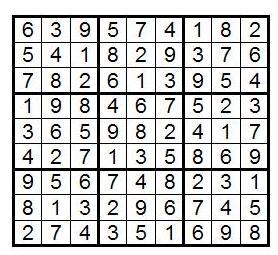
For example, in the following picture you can see an example of sudoku, as well as its decision:
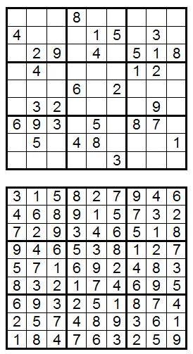
They say that math is not needed to solve Sudoku - this is not true. It actually means that only arithmetic is not needed. The puzzle does not depend on the fact that we use numbers from 1 to 9. We can easily replace these 9 numbers with letters, colors or sushi . In fact, to solve Sudoku you need to apply this kind of mathematical thinking, like logical deduction.
The simplest heuristics for solving sudoku is to first write out for every empty cell all possible numbers that can be written there, without contradicting the General Rule, using the numbers given initially. If only one option is possible for a cell, it is this one that needs to be written in this cell.
Another approach to solve is to choose a number, and after that a row, column or block. After that, you should consider all the positions in the row / column / block and check whether the selected number can be placed there without breaking the Main Rule. If the number is suitable for only one position - you can safely enter it there. Once this is done, the selected number can be excluded from the possible options for all other empty cells in the corresponding row, column, and block.
Usually these two rules are not enough to fill the net with sudoku. Often, more sophisticated methods are required to achieve progress, and sometimes it is necessary to go through the options and roll back if the selection fails. A more sophisticated strategy is to look at pairs or triples of cells in a row, column, or block. It may turn out that for the pair of cells in question only two numbers from the group are suitable, but it is unclear which of them should be placed in which of these two cells. However, from this we can conclude that the numbers from this pair cannot appear on any other places in the group in question. This reduces the number of options in other empty cells and helps get closer to the solution. Similarly, if a triple of numbers can be placed only in a certain triple of positions (not clearly in what order), then these three numbers can be excluded from consideration for all other cells in the neighborhood.
Note that in addition to the data heuristics there are many others. You can even come up with your own solution strategies.
When none of the simple heuristics helps, you need to try to select an empty cell with the fewest options and try one of the options. In the case of a contradiction (repeated numbers in a row, column or block), you should cancel all your actions until the moment of your choice and try another option.
Exercise: Try the above methods on this sudoku:
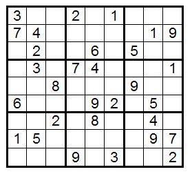
On the Internet you can find many other sudoku of any complexity and for every taste.
This is a very interesting question. So how many different sudoku are 9 × 9? How many ways can you fill a 9 × 9 table with numbers from 1 to 9 so that the Main Rule is fulfilled? We describe the method by which Bertram Felgenhauer and Frazer Jarvis calculated this number at the beginning of 2006.
First agree on the notation. We will call a strip a triple of blocks whose centers are located on the same horizontal line. Total we have three bands - top, bottom and middle. A stack will be called a triple of blocks whose centers are located on the same vertical. We also have three stacks, like the bands, left, right and middle. The cell at the intersection of the i-th row and j-th column will be denoted as (i, j) .
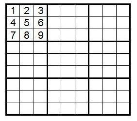
Preparations are over and we are ready to count the number N - the number of different sudoku. First, we denote all sudoku blocks as follows:
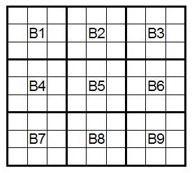
How many ways can I fill in block B1? Since for block B1 we have 9 numbers, one for each cell, in the first one we can write one of the numbers in one of 9 ways. For each of these 9 ways, we have 8 ways to place one of the remaining numbers in exactly 8 ways. For the third cell for each of these 9 × 8 ways, the number of options to go further is exactly 7. We are, in fact, trying to build all possible permutations of length 9 and the number of ways we need to fill the B1 block is equal to the number of these permutations - 9! = 9 × 8 × 7 × 6 × 7 × 4 × 3 × 2 × 1 = 362880. Starting from sudoku, in which block B1 is filled in a certain way, we can get sudoku with any other filling of block B1 by simply reassigning numbers ( recall that it doesn’t matter to us what numbers are where - the main thing is to know where the numbers are the same and where are different ) Therefore, for simplicity, fill the block B1 with numbers from 1 to 9 in the order shown in the figure:
Let the number of sudoku in which block B1 is filled exactly as in the picture is N1. The total number of sudoku will be N1 × 9!, Hence N1 = N / 9 !.
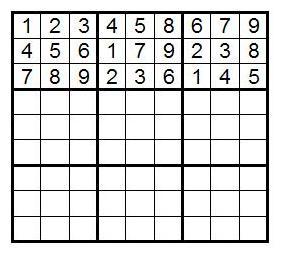
Consider all the ways to fill the first row in blocks B2 and B3. Since 1, 2 and 3 are already present in block B1, these numbers can no longer be used in this string. Only the numbers 4, 5, 6, 7, 8 and 9 from the second and third lines of block B1 can be used in the first line of blocks B2 and B3.
Exercise: List all possible ways to fill the first line in blocks B2 and B3 with permutation accuracy. Hint: there are a total of ten ways to split six numbers into two parts of three, and changing B2 to B3, we get ten more ways. Total - twenty.
Let us call two of these options pure upper lines : when the numbers {4,5,6}, as in the second row of block B1, are placed together in B2, and the numbers {7,8,9}, as in the third row of block B1, are arranged together in B3 (well, the case when B2 and B3 are swapped). All other methods are mixed upper lines , since in the first line B2 and B3, the sets {4,5,6} and {7,8,9} are mixed together.
Well, we have these twenty ways, and we want to know how to fill in the remaining cells in the front page.
Exercise: Think a little about how you can fill in the first lane starting with a clean top line 1,2,3; {4,5,6}; {7,8,9} (we write a, b, c, if there are three numbers go in fixed order and {a, b, c} if these numbers can go in any order). How many ways are there, considering the different ordering methods in B2 and B3? It is true that there are as many of these methods as for the other clean row 1,2,3; {7,8,9}; {4,5,6}?
Remember, we do not change the order in block B1, since we already take into account the number of grids, which are obtained by mixing devies of numbers in B1.
It turns out that for a clean top line 1,2,3; {4,5,6}; {7,8,9} - exactly (3!) 6 ways, because we definitely need to put {7,8,9}; { 1,2,3} on the second line in blocks B2 and B3, and {1,2,3}; {4,5,6} - on the third line. After that, we can randomly swap the numbers in these six triples in B2 and B3 in order to get all the configurations. For the second clean top line, the answer is the same, since all that we change places is blocks B2 and B3.
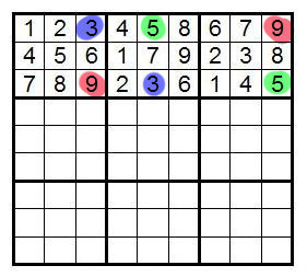
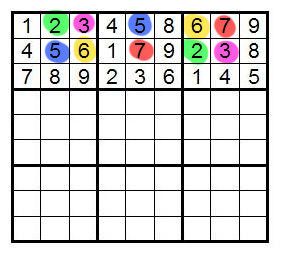
For the case of mixed top lines, everything is more complicated. Let's look at the top row 1,2,3; {4,6,8}; {5,7,9}. Further, the first lane can be filled as shown in the picture below, where a, b and c are the numbers 1, 2, 3 in any order.
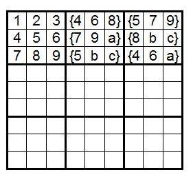
As soon as the number a is chosen, b and c are the remaining two numbers in any order, since they are in the same lines. For a, there are three ways to choose, and then we can simply mix the numbers in six triples in B2 and B3 in any order — and you will always get a suitable front page. Total number of configurations - 3x (3!) 6 . It is easy to show that in the remaining seventeen ways we get the same number.
Now we can calculate the total number of different upper bands for a fixed block B1: 2x (3!) 6 + 18x3x (3!) 6 = 2612736. The first part of the sum is the number of lanes for the net upper lanes, and the second - for the mixed ones.
Instead of counting the number of different fully filled grids for each of these 2,612,736 options, Felgenhauer and Jarvis first determined which of these upper bands had the same number of full fill options. This analysis reduces the number of bands that we will need to consider for further calculations.
There are several operations that leave the number of completely filled grids unchanged: reassign numbers, swap any blocks in the first lane, shuffle the columns in any block, change the order of three lines in the lane. As soon as any of the operations change the order of the numbers in B1, we simply reassign the numbers so as to bring the B1 block to a standard form.
When we swap the blocks B1, B2 and B3 - the number of fillings of the grids is preserved, since we start with the correct grid of sudoku, and the only way to maintain correctness in the future is to swap B4, B5, B6 and B7, B8, B9 as we changed B1, B2, B3. In the end, all the stacks will remain the same. In other words, each correct filling of the entire grid for one upper strip gives exactly one correct filling of the grid for the other upper strip obtained by mixing blocks B1, B2, B3.
Exercise: See for yourself that if you swap blocks B2 and B3 in the next grid, the only way to keep the grid correct is to swap B5 and B6, and also B8 and B9. The stacks remain the same, but their locations change.
Exercise: Suppose you have a correctly filled sudoku grid and you swap some columns in any of the blocks B1, B2 or B3. What needs to be done additionally with the remaining columns so that the Sudoku grid remains correct? For example, if you swapped the first and second columns in block B2, how would you correct the rest of the grid so that it still satisfies the Main Rule?
The last exercise tells us that each filling of the first bar gives us a unique filling for such a first bar, in which the columns are arranged in a certain way inside the blocks.
This observation allows us to reduce the number of front pages that we need to consider. According to Felgenhauer and Jarvis, we shuffle the columns in blocks B2 and B3 so that the values in the topmost row go in ascending order. After that, we may swap blocks B2 and B3 so that the very first number in block B2 ( upper left ) is less than the very first number in block B3. This operation is called lexicographic reduction. Since for each of the two blocks we have exactly 6 different permutations and only 2 ways to arrange the blocks relative to each other, the lexicographic reduction tells us that for any first lane you can build a class of 6 2 × 2 = 72 first lanes with the same number full fillings of grids ( and for all elements from each class this construction will lead to the same class ). Thus, we now need to consider only 2612736/72 = 36288 front pages.
For each of these options, we consider all sorts of permutations of the three upper blocks: there are exactly 6. And for each of these options, there are 6 3 permutations of columns inside all the blocks. After we mix everything up, you reassign the numbers so that in block B1 they all go in the standard order. We can also randomly shuffle the top three lines, then reassign the numbers again so that the B1 block becomes standard. After each of these operations, the amount of filling in the entire grid for this first band will remain unchanged. Felgenhauer and Jarvis, using a computer program, determined that these operations reduce the number of front pages that it makes sense to consider, from 36,288 to only 416.
Exercise: Consider a defined front page. Do some operations on it that save the number of fillings for the entire sudoku grid. You can start with the following: swap the first and second lines. After that, reassign the numbers in block B1 to bring it to standard form. Perform lexicographic reduction.
The main thing you should pay attention to is: the band with which we started and the band with which we finished have the same amount of filling the entire grid with sudoku. Therefore, instead of calculating the number of fillings of the grids for each band, we can count their number only for one of them.
There are several more operations that reduce the number of grids to consider. If we have a pair of numbers {a, b} such that a and b are in the same column, moreover, a is on the i-th line, and b is on the j-th, and, among other things, there is the same pair in another column, and for this column a is already on the j-th row, and b is on the i-th row ( i.e., these four numbers are in the corners of a rectangle, and the opposite numbers are equal ), then we can swap numbers in both pairs and get a new correct band with the same number of finite grids. For example, in Sudoku, just above, the numbers 8 and 9 in the sixth and ninth columns form this configuration. Having considered all possible cases, Felgenhauer and Jarvis reduced the number of front pages needed for consideration from 416 to 174.
But that's not all. They considered other configurations of the same sets ( of three or more numbers ) lying opposite each other in two different columns or rows that can be swapped and the response will not change. This reduces the number of options to 71, and if we further consider these options and apply more complex symmetries there, the number of bands for consideration can be reduced to 44. And for each of these 44 bands, all the other bands in the corresponding class have the same number of complete fillings of the entire grid. .
Let C be one of 44 bands. Then the number of ways in which C can be added to the full grid of sudoku is denoted by n C. We will also need the number m C - the total number of lanes for which the number of final fillings is the same as that of C. When the total number of different sudoku is N = Σ C m C n C , that is, the sum of m C n C over all 44 lanes.
Felgenhauer and Jarvis wrote a computer program to perform the final calculations. They calculated the number N1 (the number of correct fillings, in which B1 is in standard form) for each of the 44 bands. Then they multiplied that number by 9! To get an answer. They found that the number of all possible correct sudoku grids 9 by 9 is equal to N = 6670903752021072936960, which is approximately equal to 6.671 × 10 21 .
In the next part, we count the number of really different sudoku, assuming that two sudoku are the same if they turn into each other by turns, reflections, shuffling of columns, and so on. To do this, we dive into the theory of groups, get acquainted with the Burnside Lemma and, of course, write an hellish program to calculate the answer. In general, do not miss.
Unfortunately, the original of this article was written for
Introduction
Sudoku is a puzzle that has gained worldwide popularity since 2005. In order to solve Sudoku, we need only logic and trial and error. Complicated maths appear only on closer examination: to calculate the number of different grids, sudoku needs combinatorics to determine the number of these grids without taking into account all possible symmetries you need group theory, and to solve sudoku on an industrial scale - the theory of complexity of algorithms.
')
For the first time, the Sudoku puzzle in a form known to us was published in 1979 in the American magazine Dell Magazines under the name “Numbers in Place” by Howard Garns. In 1984, Sudoku was first published in Japan in the journal Nikoli. It was Maki Kaji, president of Nikoli (which, by the way, specializes in all kinds of puzzles and logic games), gave the puzzle the name “sudoku”, which in Japanese means “single numbers”. When the game became popular in Japan, it was New Zealander Wayne Gould who drew attention to it. Wayne wrote a program that could generate hundreds of sudoku. In 2004, he published some of these puzzles in London newspapers. Shortly thereafter, a fever of sudoku swept across England. In 2005, the puzzle became popular in the United States. Sudoku began to be published regularly in many newspapers and magazines, delighting people around the world.
The classic version of Sudoku has the form of a square table 9 × 9, total - 81 cells . This table is divided into 9 3 × 3 blocks . Some cells contain numbers from the set {1,2,3,4,5,6,7,8,9} (these numbers cannot be changed), the remaining cells are empty. The goal of the game is to fill all empty cells using only the above nine numbers, so that on each horizontal line, on each vertical, and also on each block, each of the numbers would be present exactly once. We will call these restrictions the Main Rule of the game.
The rules described above refer to sudoku of order 3. In the general case, sudoku of order n is a table n 2 × n 2 divided into n 2 blocks of size n × n each. And all this needs to be filled with numbers from 1 to n 2 so that the Main Rule is fulfilled.
For example, in the following picture you can see an example of sudoku, as well as its decision:
Approaches to the solution
They say that math is not needed to solve Sudoku - this is not true. It actually means that only arithmetic is not needed. The puzzle does not depend on the fact that we use numbers from 1 to 9. We can easily replace these 9 numbers with letters, colors or sushi . In fact, to solve Sudoku you need to apply this kind of mathematical thinking, like logical deduction.
The simplest heuristics for solving sudoku is to first write out for every empty cell all possible numbers that can be written there, without contradicting the General Rule, using the numbers given initially. If only one option is possible for a cell, it is this one that needs to be written in this cell.
Another approach to solve is to choose a number, and after that a row, column or block. After that, you should consider all the positions in the row / column / block and check whether the selected number can be placed there without breaking the Main Rule. If the number is suitable for only one position - you can safely enter it there. Once this is done, the selected number can be excluded from the possible options for all other empty cells in the corresponding row, column, and block.
Usually these two rules are not enough to fill the net with sudoku. Often, more sophisticated methods are required to achieve progress, and sometimes it is necessary to go through the options and roll back if the selection fails. A more sophisticated strategy is to look at pairs or triples of cells in a row, column, or block. It may turn out that for the pair of cells in question only two numbers from the group are suitable, but it is unclear which of them should be placed in which of these two cells. However, from this we can conclude that the numbers from this pair cannot appear on any other places in the group in question. This reduces the number of options in other empty cells and helps get closer to the solution. Similarly, if a triple of numbers can be placed only in a certain triple of positions (not clearly in what order), then these three numbers can be excluded from consideration for all other cells in the neighborhood.
Note that in addition to the data heuristics there are many others. You can even come up with your own solution strategies.
When none of the simple heuristics helps, you need to try to select an empty cell with the fewest options and try one of the options. In the case of a contradiction (repeated numbers in a row, column or block), you should cancel all your actions until the moment of your choice and try another option.
Exercise: Try the above methods on this sudoku:
On the Internet you can find many other sudoku of any complexity and for every taste.
So how many of them?
This is a very interesting question. So how many different sudoku are 9 × 9? How many ways can you fill a 9 × 9 table with numbers from 1 to 9 so that the Main Rule is fulfilled? We describe the method by which Bertram Felgenhauer and Frazer Jarvis calculated this number at the beginning of 2006.
First agree on the notation. We will call a strip a triple of blocks whose centers are located on the same horizontal line. Total we have three bands - top, bottom and middle. A stack will be called a triple of blocks whose centers are located on the same vertical. We also have three stacks, like the bands, left, right and middle. The cell at the intersection of the i-th row and j-th column will be denoted as (i, j) .
Preparations are over and we are ready to count the number N - the number of different sudoku. First, we denote all sudoku blocks as follows:
How many ways can I fill in block B1? Since for block B1 we have 9 numbers, one for each cell, in the first one we can write one of the numbers in one of 9 ways. For each of these 9 ways, we have 8 ways to place one of the remaining numbers in exactly 8 ways. For the third cell for each of these 9 × 8 ways, the number of options to go further is exactly 7. We are, in fact, trying to build all possible permutations of length 9 and the number of ways we need to fill the B1 block is equal to the number of these permutations - 9! = 9 × 8 × 7 × 6 × 7 × 4 × 3 × 2 × 1 = 362880. Starting from sudoku, in which block B1 is filled in a certain way, we can get sudoku with any other filling of block B1 by simply reassigning numbers ( recall that it doesn’t matter to us what numbers are where - the main thing is to know where the numbers are the same and where are different ) Therefore, for simplicity, fill the block B1 with numbers from 1 to 9 in the order shown in the figure:
Let the number of sudoku in which block B1 is filled exactly as in the picture is N1. The total number of sudoku will be N1 × 9!, Hence N1 = N / 9 !.
Consider all the ways to fill the first row in blocks B2 and B3. Since 1, 2 and 3 are already present in block B1, these numbers can no longer be used in this string. Only the numbers 4, 5, 6, 7, 8 and 9 from the second and third lines of block B1 can be used in the first line of blocks B2 and B3.
Exercise: List all possible ways to fill the first line in blocks B2 and B3 with permutation accuracy. Hint: there are a total of ten ways to split six numbers into two parts of three, and changing B2 to B3, we get ten more ways. Total - twenty.
Let us call two of these options pure upper lines : when the numbers {4,5,6}, as in the second row of block B1, are placed together in B2, and the numbers {7,8,9}, as in the third row of block B1, are arranged together in B3 (well, the case when B2 and B3 are swapped). All other methods are mixed upper lines , since in the first line B2 and B3, the sets {4,5,6} and {7,8,9} are mixed together.
Well, we have these twenty ways, and we want to know how to fill in the remaining cells in the front page.
Exercise: Think a little about how you can fill in the first lane starting with a clean top line 1,2,3; {4,5,6}; {7,8,9} (we write a, b, c, if there are three numbers go in fixed order and {a, b, c} if these numbers can go in any order). How many ways are there, considering the different ordering methods in B2 and B3? It is true that there are as many of these methods as for the other clean row 1,2,3; {7,8,9}; {4,5,6}?
Remember, we do not change the order in block B1, since we already take into account the number of grids, which are obtained by mixing devies of numbers in B1.
It turns out that for a clean top line 1,2,3; {4,5,6}; {7,8,9} - exactly (3!) 6 ways, because we definitely need to put {7,8,9}; { 1,2,3} on the second line in blocks B2 and B3, and {1,2,3}; {4,5,6} - on the third line. After that, we can randomly swap the numbers in these six triples in B2 and B3 in order to get all the configurations. For the second clean top line, the answer is the same, since all that we change places is blocks B2 and B3.
For the case of mixed top lines, everything is more complicated. Let's look at the top row 1,2,3; {4,6,8}; {5,7,9}. Further, the first lane can be filled as shown in the picture below, where a, b and c are the numbers 1, 2, 3 in any order.
As soon as the number a is chosen, b and c are the remaining two numbers in any order, since they are in the same lines. For a, there are three ways to choose, and then we can simply mix the numbers in six triples in B2 and B3 in any order — and you will always get a suitable front page. Total number of configurations - 3x (3!) 6 . It is easy to show that in the remaining seventeen ways we get the same number.
Now we can calculate the total number of different upper bands for a fixed block B1: 2x (3!) 6 + 18x3x (3!) 6 = 2612736. The first part of the sum is the number of lanes for the net upper lanes, and the second - for the mixed ones.
Instead of counting the number of different fully filled grids for each of these 2,612,736 options, Felgenhauer and Jarvis first determined which of these upper bands had the same number of full fill options. This analysis reduces the number of bands that we will need to consider for further calculations.
There are several operations that leave the number of completely filled grids unchanged: reassign numbers, swap any blocks in the first lane, shuffle the columns in any block, change the order of three lines in the lane. As soon as any of the operations change the order of the numbers in B1, we simply reassign the numbers so as to bring the B1 block to a standard form.
When we swap the blocks B1, B2 and B3 - the number of fillings of the grids is preserved, since we start with the correct grid of sudoku, and the only way to maintain correctness in the future is to swap B4, B5, B6 and B7, B8, B9 as we changed B1, B2, B3. In the end, all the stacks will remain the same. In other words, each correct filling of the entire grid for one upper strip gives exactly one correct filling of the grid for the other upper strip obtained by mixing blocks B1, B2, B3.
Exercise: See for yourself that if you swap blocks B2 and B3 in the next grid, the only way to keep the grid correct is to swap B5 and B6, and also B8 and B9. The stacks remain the same, but their locations change.
Exercise: Suppose you have a correctly filled sudoku grid and you swap some columns in any of the blocks B1, B2 or B3. What needs to be done additionally with the remaining columns so that the Sudoku grid remains correct? For example, if you swapped the first and second columns in block B2, how would you correct the rest of the grid so that it still satisfies the Main Rule?
The last exercise tells us that each filling of the first bar gives us a unique filling for such a first bar, in which the columns are arranged in a certain way inside the blocks.
This observation allows us to reduce the number of front pages that we need to consider. According to Felgenhauer and Jarvis, we shuffle the columns in blocks B2 and B3 so that the values in the topmost row go in ascending order. After that, we may swap blocks B2 and B3 so that the very first number in block B2 ( upper left ) is less than the very first number in block B3. This operation is called lexicographic reduction. Since for each of the two blocks we have exactly 6 different permutations and only 2 ways to arrange the blocks relative to each other, the lexicographic reduction tells us that for any first lane you can build a class of 6 2 × 2 = 72 first lanes with the same number full fillings of grids ( and for all elements from each class this construction will lead to the same class ). Thus, we now need to consider only 2612736/72 = 36288 front pages.
Comment
I think it's time to start writing code to make the article a little more hardcore. We are going to check that the lexicographically reduced upper lanes, in which the block B1 is standard - exactly 36,288 pieces.
To begin with, we will describe the structure for our band (I, as usual, write in C ++):
The code of explanations deserves only the is_valid () method: it checks that the Main Rule for the strip is executed. If the with_zeros argument is true, then the method does not take into account zeros (and with zeros we will denote cells of partially filled bands, in which no digit has yet been assigned).
The code for generating all the bands we are interested in is as follows:
First we prepare the starting_bands - the bands in which block B1 is filled and the first lines of blocks B2 and B3. There are only 10 of them, because in order to maintain the lexicographical order, we do not take into account options when block B2 is “larger” than block B3. After this, we simply search through all the required bands. The calculations given above in the code are not used - they are more for the "head" than for the machine. The main thing is that the numbers eventually came together. And we will use the generated bands later in the next spoiler.
To begin with, we will describe the structure for our band (I, as usual, write in C ++):
struct BAND { int m[3][3][3]; // 3 blocks of 3x3 grids BAND() { for (int i=0; i<3; i++) for (int j=0; j<3; j++) for (int k=0; k<3; k++) m[i][j][k] = 0; } void print() { for (int i=0; i<3; i++) { for (int j=0; j<3; j++) { for (int k=0; k<3; k++) printf( "%d", m[j][i][k] ); printf( " " ); } printf( "\n" ); } printf( "\n" ); } bool is_valid( bool with_zeros ) { for (int i=0; i<3; i++) for (int j=0; j<3; j++) for (int k=0; k<3; k++) { if (!(0<=m[i][j][k] && m[i][j][k]<=9)) return false; if (!with_zeros && m[i][j][k]==0) return false; } bool F[10]; for (int i=0; i<3; i++) // check blocks { memset( F, 0, sizeof( F ) ); for (int j=0; j<3; j++) for (int k=0; k<3; k++) { if (F[m[i][j][k]]) return false; if (m[i][j][k]>0) F[m[i][j][k]] = true; } } for (int i=0; i<3; i++) // check rows { memset( F, 0, sizeof( F ) ); for (int j=0; j<3; j++) for (int k=0; k<3; k++) { if (F[m[j][i][k]]) return false; if (m[j][i][k]>0) F[m[j][i][k]] = true; } } return true; } }; The code of explanations deserves only the is_valid () method: it checks that the Main Rule for the strip is executed. If the with_zeros argument is true, then the method does not take into account zeros (and with zeros we will denote cells of partially filled bands, in which no digit has yet been assigned).
The code for generating all the bands we are interested in is as follows:
void gen_bands( BAND band, int block, int row, int col, vector< BAND > & res ) { col++; // move to the next empty cell if (col==3) { col=0; row++; } if (row==3) { row=1; block++; } if (block==3) // no next empty cell { res.push_back( band ); return; } for (int a=1; a<=9; a++) { band.m[block][row][col] = a; if (band.is_valid( true )) gen_bands( band, block, row, col, res ); } } vector< BAND > gen_all_bands() { BAND b0; int t=1; for (int i=0; i<3; i++) for (int j=0; j<3; j++) b0.m[0][i][j] = t++; // b0 has standard block B1; B2 and B3 are empty vector< BAND > starting_bands; for (int a=4; a<=4; a++) for (int b=a+1; b<=9; b++) for (int c=b+1; c<=9; c++) { BAND b1 = b0; b1.m[1][0][0] = a; b1.m[1][0][1] = b; b1.m[1][0][2] = c; int ind = 0; for (int d=4; d<=9; d++) if (d!=a && d!=b && d!=c) b1.m[2][0][ind++] = d; //b1.print(); starting_bands.push_back( b1 ); } // we filled the first row by all possible ways printf( "bands with filled the first row %d\n", (int)starting_bands.size() ); // 10 bands total vector< BAND > reduced_bands; for (int i=0; i<(int)starting_bands.size(); i++) gen_bands( starting_bands[i], 0, 2, 2, reduced_bands ); printf( "lexicographically reduced bands %d\n", (int)reduced_bands.size() ); // 36288 bands total return reduced_bands; } First we prepare the starting_bands - the bands in which block B1 is filled and the first lines of blocks B2 and B3. There are only 10 of them, because in order to maintain the lexicographical order, we do not take into account options when block B2 is “larger” than block B3. After this, we simply search through all the required bands. The calculations given above in the code are not used - they are more for the "head" than for the machine. The main thing is that the numbers eventually came together. And we will use the generated bands later in the next spoiler.
For each of these options, we consider all sorts of permutations of the three upper blocks: there are exactly 6. And for each of these options, there are 6 3 permutations of columns inside all the blocks. After we mix everything up, you reassign the numbers so that in block B1 they all go in the standard order. We can also randomly shuffle the top three lines, then reassign the numbers again so that the B1 block becomes standard. After each of these operations, the amount of filling in the entire grid for this first band will remain unchanged. Felgenhauer and Jarvis, using a computer program, determined that these operations reduce the number of front pages that it makes sense to consider, from 36,288 to only 416.
Exercise: Consider a defined front page. Do some operations on it that save the number of fillings for the entire sudoku grid. You can start with the following: swap the first and second lines. After that, reassign the numbers in block B1 to bring it to standard form. Perform lexicographic reduction.
The main thing you should pay attention to is: the band with which we started and the band with which we finished have the same amount of filling the entire grid with sudoku. Therefore, instead of calculating the number of fillings of the grids for each band, we can count their number only for one of them.
Comment
From this point on, some non-obviousness begins - the authors of the original offer to believe them in word. But we are not like that - we will write code to make sure in person. Namely: now we will check the fact that by performing the operations described above, we will end up with exactly 416 options.
For greater clarity, let us describe what we will do now: we will build a graph. Imagine that each of the lexicographically reduced bands is a vertex of a graph (that is, we have only 36,288 vertices). When we apply an operation to a strip (which mixes numbers, but does not change the number of final grids for a given strip) - we in our graph connect the starting strip and the ending strip with an edge. The edges are undirected, since each of the above operations is reversible - we can return everything backwards by doing the actions in the reverse order. Now let's apply all sorts of operations for each strip and draw all sorts of edges. Then, for any two vertices connected by a chain of edges, the answer will be the same. Anyway, it will be the same for all vertices in the same connected component. That is, we need to count the number of connected components in the resulting graph - and there should be exactly 416 of them.
First we make modifications to the BAND structure:
Now we can lexicographically reduce our band (the normalize () method), and also do all 3 operations described above. When applying an operation, a copy of the object is created, then an operation is applied to the copy, then the result is normalized (so as not to go beyond the reduced 36,288 bands).
Now we can calculate the number of connected components using standard depth traversal. In this case, the graph is clearly not built.
Comparison operators are needed so that they can be used by set. As a result, the program actually finds exactly 416 connectivity components. In comp_sizes, the sizes of these components are added, and in ident_bands, one of the vertices from each component (the bar is a representative of the class). It should be noted that the resulting components do not always have the same size. For example, the program displays the following dimensions:
Well, now, in fact, you can count the number of final fillings for each representative, multiply by the number of vertices in the corresponding component and at the end add up. But with this we will not hurry.
For greater clarity, let us describe what we will do now: we will build a graph. Imagine that each of the lexicographically reduced bands is a vertex of a graph (that is, we have only 36,288 vertices). When we apply an operation to a strip (which mixes numbers, but does not change the number of final grids for a given strip) - we in our graph connect the starting strip and the ending strip with an edge. The edges are undirected, since each of the above operations is reversible - we can return everything backwards by doing the actions in the reverse order. Now let's apply all sorts of operations for each strip and draw all sorts of edges. Then, for any two vertices connected by a chain of edges, the answer will be the same. Anyway, it will be the same for all vertices in the same connected component. That is, we need to count the number of connected components in the resulting graph - and there should be exactly 416 of them.
First we make modifications to the BAND structure:
struct BAND { /* old code */ void normalize() // turn into standard form { // relabeling int relabel[10]; int t = 1; for (int i=0; i<3; i++) for (int j=0; j<3; j++) relabel[m[0][i][j]] = t++; for (int i=0; i<3; i++) for (int j=0; j<3; j++) for (int k=0; k<3; k++) m[i][j][k] = relabel[m[i][j][k]]; // lexicographic reduction for (int i=1; i<3; i++) { if (m[i][0][0] > m[i][0][1]) for (int j=0; j<3; j++) swap( m[i][j][0], m[i][j][1] ); if (m[i][0][1] > m[i][0][2]) for (int j=0; j<3; j++) swap( m[i][j][1], m[i][j][2] ); if (m[i][0][0] > m[i][0][1]) for (int j=0; j<3; j++) swap( m[i][j][0], m[i][j][1] ); } // swap B2 and B3 if (m[1][0][0] > m[2][0][0]) for (int i=0; i<3; i++) for (int j=0; j<3; j++) swap( m[1][i][j], m[2][i][j] ); } BAND get_copy() { BAND re; for (int i=0; i<3; i++) for (int j=0; j<3; j++) for (int k=0; k<3; k++) re.m[i][j][k] = m[i][j][k]; return re; } BAND swap_blocks( int x, int y ) // swap blocks x and y { BAND re = get_copy(); for (int i=0; i<3; i++) for (int j=0; j<3; j++) swap( re.m[x][i][j], re.m[y][i][j] ); re.normalize(); return re; } BAND swap_rows( int x, int y ) // swap rows x and y { BAND re = get_copy(); for (int i=0; i<3; i++) for (int j=0; j<3; j++) swap( re.m[i][x][j], re.m[i][y][j] ); re.normalize(); return re; } BAND swap_columns( int b, int x, int y ) // swap columns x and y in block b { BAND re = get_copy(); for (int i=0; i<3; i++) swap( re.m[b][i][x], re.m[b][i][y] ); re.normalize(); return re; } }; Now we can lexicographically reduce our band (the normalize () method), and also do all 3 operations described above. When applying an operation, a copy of the object is created, then an operation is applied to the copy, then the result is normalized (so as not to go beyond the reduced 36,288 bands).
Now we can calculate the number of connected components using standard depth traversal. In this case, the graph is clearly not built.
bool operator< ( const BAND & A, const BAND & B ) { for (int i=0; i<3; i++) for (int j=0; j<3; j++) for (int k=0; k<3; k++) if (Am[i][j][k] != Bm[i][j][k]) return Am[i][j][k] < Bm[i][j][k]; return false; } bool operator== ( const BAND & A, const BAND & B ) { for (int i=0; i<3; i++) for (int j=0; j<3; j++) for (int k=0; k<3; k++) if (Am[i][j][k] != Bm[i][j][k]) return false; return true; } set< BAND > used_bands; int comp_size; void dfs( BAND b ) { if (used_bands.find( b ) != used_bands.end()) return; comp_size++; used_bands.insert( b ); for (int i=0; i<3; i++) for (int j=i+1; j<3; j++) { dfs( b.swap_blocks( i, j ) ); dfs( b.swap_rows( i, j ) ); for (int k=0; k<3; k++) dfs( b.swap_columns( k, i, j ) ); } } void solution() { vector< BAND > bands = gen_all_bands(); vector< int > comp_sizes; vector< BAND > ident_bands; for (int i=0; i<(int)bands.size(); i++) if (used_bands.find( bands[i] ) == used_bands.end()) { comp_size = 0; dfs( bands[i] ); comp_sizes.push_back( comp_size ); ident_bands.push_back( bands[i] ); } printf( "number of connected components %d\n", (int)comp_sizes.size() ); // 416 components for (int i=0; i<(int)comp_sizes.size(); i++) printf( "%d ", comp_sizes[i] ); } Comparison operators are needed so that they can be used by set. As a result, the program actually finds exactly 416 connectivity components. In comp_sizes, the sizes of these components are added, and in ident_bands, one of the vertices from each component (the bar is a representative of the class). It should be noted that the resulting components do not always have the same size. For example, the program displays the following dimensions:
1 27 18 54 6 9 54 108 9 54 108 54 54 108 54 54 54 18 6 108 54 54 6 18 6 54 18 54 18 54 2 54 108 108 108 54 108 108 108 108 54 108 108 108 54 108 108 54 108 54 108 54 108 108 108 54 108 108 108 54 108 108 108 54 108 108 108 108 108 108 108 108 108 108 108 108 108 108 108 108 54 108 108 108 108 108 108 108 54 108 108 108 108 54 108 108 108 18 108 108 54 108 108 108 54 54 108 108 108 54 54 108 108 108 108 108 108 108 108 108 108 108 108 108 108 108 108 108 108 54 108 108 108 108 108 108 108 108 108 108 108 108 108 108 54 54 54 18 54 54 108 108 108 108 108 108 108 108 108 108 108 108 108 108 108 108 108 108 108 108 108 54 108 108 108 108 54 108 108 54 108 108 108 108 108 108 108 108 108 36 108 108 108 108 108 108 108 108 108 108 108 108 108 108 108 54 108 54 108 108 108 108 108 108 108 54 108 108 108 54 108 108 108 108 54 108 108 108 108 108 108 108 108 108 108 108 108 108 108 108 108 108 108 108 108 108 108 108 54 108 108 54 108 108 108 108 108 54 108 108 108 108 108 108 54 54 54 54 54 54 6 18 54 18 108 54 54 108 54 54 108 54 54 108 108 108 108 54 108 108 108 108 108 54 108 108 108 108 108 108 108 54 54 108 108 108 108 108 54 108 54 108 108 54 54 108 108 108 108 108 108 54 18 18 54 54 108 54 54 108 108 54 108 108 54 108 108 108 108 108 54 108 54 18 54 108 108 54 54 108 108 54 54 108 108 108 54 54 108 108 108 108 108 108 108 54 36 108 108 108 108 108 54 108 108 108 108 108 54 108 108 54 54 108 54 108 108 108 54 54 108 108 108 54 18 108 54 54 54 108 54 18 18 54 54 54 108 18 54 54 54 54 3 27 9 9
Well, now, in fact, you can count the number of final fillings for each representative, multiply by the number of vertices in the corresponding component and at the end add up. But with this we will not hurry.
There are several more operations that reduce the number of grids to consider. If we have a pair of numbers {a, b} such that a and b are in the same column, moreover, a is on the i-th line, and b is on the j-th, and, among other things, there is the same pair in another column, and for this column a is already on the j-th row, and b is on the i-th row ( i.e., these four numbers are in the corners of a rectangle, and the opposite numbers are equal ), then we can swap numbers in both pairs and get a new correct band with the same number of finite grids. For example, in Sudoku, just above, the numbers 8 and 9 in the sixth and ninth columns form this configuration. Having considered all possible cases, Felgenhauer and Jarvis reduced the number of front pages needed for consideration from 416 to 174.
But that's not all. They considered other configurations of the same sets ( of three or more numbers ) lying opposite each other in two different columns or rows that can be swapped and the response will not change. This reduces the number of options to 71, and if we further consider these options and apply more complex symmetries there, the number of bands for consideration can be reduced to 44. And for each of these 44 bands, all the other bands in the corresponding class have the same number of complete fillings of the entire grid. .
Comment
Let's supplement our program with new operations in order to get improvements up to 174 and up to 71 lanes. We will not improve up to 44 lanes - everything is quite difficult there, and there is very little intelligible information about this. Felgenhauer and Jarvis in their article improve only to 71, and they bring the number 44 already at the end after all calculations (however, they also write that there are suitable transformations to get the required 44 bands - about this at the end of this spoiler).
So, let's add the operation of swapping two pairs of numbers, which are located in the corners of one rectangle. This is very easy to add to the code already written:
We simply iterate through all the rectangles (the only optimization is that the left and right columns of this rectangle should lie in different blocks for obvious reasons) and check that the numbers in the opposite corners are the same. If this is so, we make a change to the band, otherwise we leave the band unchanged (then, in fact, in our graph it generates a loop that does not affect anything).
If we run the updated code, we get, as expected, exactly 174 bands.
Add more operations:
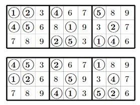
The first of the swap_3x2 () operations is the case when we look for identical subsets in two columns. The fact is that a subset of size 1 does not exist (the Main Rule is otherwise violated), a subset of size 2 is already processed by the swap_cross () procedure, and we have 3 rows in total. Hence, we need to check only one option - all three numbers in two columns. For them, there are exactly two match options:
If everything is the same, we simply swap the columns. Otherwise - leave the strip unchanged.
For the second swap_mask () operation, we iterate over various subsets of the columns and look for two rows — whether the sets of numbers for these subsets of columns are the same. Examples of suitable options:
In case of coincidence, we swap the found subsets (we match a pair in each column). If there is a mismatch, we do nothing.
It should be noted that the swap_cross () operation considered earlier is a special case of swap_mask (). Therefore, swap_cross () can be thrown out as unnecessary.
This time the launch of the program will be long - the program runs on my machine for about 30 seconds. But the result is what was expected - 71. It is clear that the code was written far from optimal, but for our purposes this performance is more than enough.
The dimensions of the connectivity components are the following:
As for the operations that reduce the number of options to 44, then they look something like this:
You can try to describe them more formally and implement in code.
So, let's add the operation of swapping two pairs of numbers, which are located in the corners of one rectangle. This is very easy to add to the code already written:
struct BAND { /* old code */ BAND swap_cross( int b1, int b2, int r1, int r2, int c1, int c2 ) { BAND re = get_copy(); // note: b1 must be together with c1 and b2 must be together with c2 if (re.m[b1][r1][c1] == re.m[b2][r2][c2] && re.m[b1][r2][c1] == re.m[b2][r1][c2]) { swap( re.m[b1][r1][c1], re.m[b2][r1][c2] ); swap( re.m[b1][r2][c1], re.m[b2][r2][c2] ); } re.normalize(); return re; } }; void dfs( BAND b ) { /* old code */ for (int b1=0; b1<3; b1++) for (int b2=b1+1; b2<3; b2++) for (int r1=0; r1<3; r1++) for (int r2=r1+1; r2<3; r2++) for (int c1=0; c1<3; c1++) for (int c2=0; c2<3; c2++) dfs( b.swap_cross( b1, b2, r1, r2, c1, c2 ) ); } We simply iterate through all the rectangles (the only optimization is that the left and right columns of this rectangle should lie in different blocks for obvious reasons) and check that the numbers in the opposite corners are the same. If this is so, we make a change to the band, otherwise we leave the band unchanged (then, in fact, in our graph it generates a loop that does not affect anything).
If we run the updated code, we get, as expected, exactly 174 bands.
Add more operations:
struct BAND { /* old code */ BAND swap_3x2( int b1, int b2, int c1, int c2 ) { BAND re = get_copy(); // note: b1 must be together with c1 and b2 must be together with c2 if (( re.m[b1][0][c1] == re.m[b2][1][c2] && re.m[b1][1][c1] == re.m[b2][2][c2] && re.m[b1][2][c1] == re.m[b2][0][c2]) || ( re.m[b1][0][c1] == re.m[b2][2][c2] && re.m[b1][1][c1] == re.m[b2][0][c2] && re.m[b1][2][c1] == re.m[b2][1][c2])) { swap( re.m[b1][0][c1], re.m[b2][0][c2] ); swap( re.m[b1][1][c1], re.m[b2][1][c2] ); swap( re.m[b1][2][c1], re.m[b2][2][c2] ); } re.normalize(); return re; } BAND swap_mask( int r1, int r2, int mask ) { BAND re = get_copy(); int num1=0, num2=0; for (int i=0; i<3; i++) // block for (int j=0; j<3; j++) // col if ((mask>>(i*3+j))&1) { num1 += (1<<re.m[i][r1][j]); num2 += (1<<re.m[i][r2][j]); } if (num1 == num2) for (int i=0; i<3; i++) // block for (int j=0; j<3; j++) // col if ((mask>>(i*3+j))&1) swap( re.m[i][r1][j], re.m[i][r2][j] ); re.normalize(); return re; } }; void dfs( BAND b ) { /* old code */ for (int b1=0; b1<3; b1++) for (int b2=b1+1; b2<3; b2++) for (int c1=0; c1<3; c1++) for (int c2=0; c2<3; c2++) dfs( b.swap_3x2( b1, b2, c1, c2 ) ); for (int r1=0; r1<3; r1++) for (int r2=r1+1; r2<3; r2++) for (int mask=1; mask<(1<<9); mask++) dfs( b.swap_mask( r1, r2, mask ) ); } The first of the swap_3x2 () operations is the case when we look for identical subsets in two columns. The fact is that a subset of size 1 does not exist (the Main Rule is otherwise violated), a subset of size 2 is already processed by the swap_cross () procedure, and we have 3 rows in total. Hence, we need to check only one option - all three numbers in two columns. For them, there are exactly two match options:
If everything is the same, we simply swap the columns. Otherwise - leave the strip unchanged.
For the second swap_mask () operation, we iterate over various subsets of the columns and look for two rows — whether the sets of numbers for these subsets of columns are the same. Examples of suitable options:
In case of coincidence, we swap the found subsets (we match a pair in each column). If there is a mismatch, we do nothing.
It should be noted that the swap_cross () operation considered earlier is a special case of swap_mask (). Therefore, swap_cross () can be thrown out as unnecessary.
This time the launch of the program will be long - the program runs on my machine for about 30 seconds. But the result is what was expected - 71. It is clear that the code was written far from optimal, but for our purposes this performance is more than enough.
The dimensions of the connectivity components are the following:
4 108 72 216 24 216 216 2592 216 216 1296 1404 540 108 72 510 702 270 2214 6 504 6 1350 666 702 18 756 20 2268 1134 2592 972 270 864 864 972 2052 486 270 1620 540 432 144 432 864 324 540 270 270 234 6 18 540 288 216 54 108 108 288 54 378 108 108 54 108 54 108 36 108 54 54
As for the operations that reduce the number of options to 44, then they look something like this:
You can try to describe them more formally and implement in code.
Let C be one of 44 bands. Then the number of ways in which C can be added to the full grid of sudoku is denoted by n C. We will also need the number m C - the total number of lanes for which the number of final fillings is the same as that of C. When the total number of different sudoku is N = Σ C m C n C , that is, the sum of m C n C over all 44 lanes.
Felgenhauer and Jarvis wrote a computer program to perform the final calculations. They calculated the number N1 (the number of correct fillings, in which B1 is in standard form) for each of the 44 bands. Then they multiplied that number by 9! To get an answer. They found that the number of all possible correct sudoku grids 9 by 9 is equal to N = 6670903752021072936960, which is approximately equal to 6.671 × 10 21 .
Comment
Let's and we will add our program for calculations. Let's start with the GRID structure - sudoku grids into which numbers can be entered and for each empty cell it is possible to find out whether it is possible to write a number into it or not.
Arrays of flags R, C, and B store information about which numbers are already marked in the corresponding rows, columns, and blocks. This then allows you to quickly determine whether you can put a number in a cell or not.
The following procedure for each band BAND builds the initial grid for iterating over the GRID and starts the iteration:
In fact, this procedure at the very beginning fills the first column of the grid, and not by all means, but only lexicographically reduced - this reduces further enumeration exactly 72 times (the main thing then is not to forget to multiply the answer by 72). Total each process_band () procedure call runs dfs2 () exactly 10 times.
The search itself looks like this:
Brute force is completely unsophisticated. We iterate over all the remaining empty cells in the following order: first, go down the second column from the top down (in blocks B4 and B7), then go down the third column from the top down, and so on.
One run of dfs2 () on my machine takes about 30 seconds, i.e. processing of one strip takes about 5 minutes. Implementation, of course, can be a little faster, you can try to do it yourself. The Felgenhauer and Jarvis program for one lane works for about 2 minutes (as they write in their article), i.e. only 2.5 times faster than our implementation. Full processing of all 71 bands (for our program) takes 6 hours.
As a result, the program displays the following:
To get the final result, you need to use a calculator (I didn't want to write long arithmetic), and ... everything is the same! You can check the numbers with those that have turned out to Felgenhauer and Jarvis here .
The full code of our program (not to collect pieces of spoilers) is here .
struct GRID { int T[9][9]; bool R[9][10], C[9][10], B[9][10]; void clear() { memset( T, 0, sizeof( T ) ); memset( R, 0, sizeof( R ) ); memset( C, 0, sizeof( C ) ); memset( B, 0, sizeof( B ) ); } void print() { for (int i=0; i<9; i++) { for (int j=0; j<9; j++) printf( "%d", T[i][j] ); printf( "\n" ); } printf( "\n" ); } bool can_set( int num, int x, int y ) { return !R[x][num] && !C[y][num] && !B[(x/3)*3+(y/3)][num]; } void set_num( int num, int x, int y ) { T[x][y] = num; R[x][num] = true; C[y][num] = true; B[(x/3)*3+(y/3)][num] = true; } void unset_num( int num, int x, int y ) { T[x][y] = 0; R[x][num] = false; C[y][num] = false; B[(x/3)*3+(y/3)][num] = false; } } G; Arrays of flags R, C, and B store information about which numbers are already marked in the corresponding rows, columns, and blocks. This then allows you to quickly determine whether you can put a number in a cell or not.
The following procedure for each band BAND builds the initial grid for iterating over the GRID and starts the iteration:
long long process_band( BAND band ) { int nums[] = { 2, 3, 5, 6, 8, 9 }; long long res = 0; for (int i=1; i<6; i++) for (int j=i+1; j<6; j++) { G.clear(); for (int a=0; a<3; a++) for (int b=0; b<3; b++) for (int c=0; c<3; c++) G.set_num( band.m[a][b][c], b, a*3+c ); G.set_num( nums[0], 3, 0 ); G.set_num( nums[i], 4, 0 ); G.set_num( nums[j], 5, 0 ); int t = 6; for (int k=1; k<6; k++) if (k!=i && k!=j) G.set_num( nums[k], t++, 0 ); // starting grid is complete //G.print(); grids_count = 0; dfs2( 8, 0 ); res += grids_count; fprintf( stderr, "." ); } return res; } In fact, this procedure at the very beginning fills the first column of the grid, and not by all means, but only lexicographically reduced - this reduces further enumeration exactly 72 times (the main thing then is not to forget to multiply the answer by 72). Total each process_band () procedure call runs dfs2 () exactly 10 times.
The search itself looks like this:
int grids_count; void dfs2( int x, int y ) { x++; // find next empty cell if (x==9) { x=3; y++; } if (y==9) // no empty cells { grids_count++; return; } for (int a=1; a<=9; a++) if (G.can_set( a, x, y )) { G.set_num( a, x, y ); dfs2( x, y ); G.unset_num( a, x, y ); } } Brute force is completely unsophisticated. We iterate over all the remaining empty cells in the following order: first, go down the second column from the top down (in blocks B4 and B7), then go down the third column from the top down, and so on.
One run of dfs2 () on my machine takes about 30 seconds, i.e. processing of one strip takes about 5 minutes. Implementation, of course, can be a little faster, you can try to do it yourself. The Felgenhauer and Jarvis program for one lane works for about 2 minutes (as they write in their article), i.e. only 2.5 times faster than our implementation. Full processing of all 71 bands (for our program) takes 6 hours.
As a result, the program displays the following:
bands with filled the first row 10 lexicographically reduced bands 36288 number of connected components 71 0/71 4 x 108374976 1/71 108 x 102543168 2/71 72 x 100231616 3/71 216 x 99083712 4/71 24 x 97282720 5/71 216 x 102047904 6/71 216 x 98875264 7/71 2592 x 98733568 8/71 216 x 98875264 9/71 216 x 99525184 10/71 1296 x 98369440 11/71 1404 x 97287008 12/71 540 x 98128064 13/71 108 x 98128064 14/71 72 x 97685328 15/71 510 x 98950072 16/71 702 x 98153104 17/71 270 x 97961464 18/71 2214 x 97961464 19/71 6 x 98950072 20/71 504 x 97685328 21/71 6 x 99258880 22/71 1350 x 97477096 23/71 666 x 97549160 24/71 702 x 97477096 25/71 18 x 97549160 26/71 756 x 96702240 27/71 20 x 94888576 28/71 2268 x 97116296 29/71 1134 x 98371664 30/71 2592 x 97539392 31/71 972 x 97910032 32/71 270 x 98493856 33/71 864 x 98119872 34/71 864 x 98733184 35/71 972 x 97116296 36/71 2052 x 96482296 37/71 486 x 97346960 38/71 270 x 97346960 39/71 1620 x 97416016 40/71 540 x 97455648 41/71 432 x 98784768 42/71 144 x 101131392 43/71 432 x 97992064 44/71 864 x 97756224 45/71 324 x 96380896 46/71 540 x 97910032 47/71 270 x 97416016 48/71 270 x 97714592 49/71 234 x 96100688 50/71 6 x 99258880 51/71 18 x 96100688 52/71 540 x 96482296 53/71 288 x 96807424 54/71 216 x 97372400 55/71 54 x 97714592 56/71 108 x 97372400 57/71 108 x 95596592 58/71 288 x 96631520 59/71 54 x 95596592 60/71 378 x 95596592 61/71 108 x 96482296 62/71 108 x 96482296 63/71 54 x 98371664 64/71 108 x 97455648 65/71 54 x 97416016 66/71 108 x 97287008 67/71 36 x 97372400 68/71 108 x 98048704 69/71 54 x 98493856 70/71 54 x 98153104 total number of sudoku 3546146300288*9!*72*72 total time 21213 sec To get the final result, you need to use a calculator (I didn't want to write long arithmetic), and ... everything is the same! You can check the numbers with those that have turned out to Felgenhauer and Jarvis here .
The full code of our program (not to collect pieces of spoilers) is here .
To be continued
In the next part, we count the number of really different sudoku, assuming that two sudoku are the same if they turn into each other by turns, reflections, shuffling of columns, and so on. To do this, we dive into the theory of groups, get acquainted with the Burnside Lemma and, of course, write an hellish program to calculate the answer. In general, do not miss.
Source: https://habr.com/ru/post/313224/
All Articles