Kinematics modeling is not difficult

I have long wanted to do the creation of robots, but there is always not enough free money, time or space. That's why I was going to write their virtual models!

Powerful tools that allow you to do this are either difficult to dock with third-party programs ( Modelica ), or proprietary (Wolfram Mathematica, various CAD systems), and I decided to make a bike on Julia . Then all the developments can be docked with the ROS services.

We assume that our robots move rather slowly and their mechanics are in the state with the lowest energy, with the constraints specified by the design and servo drives. Thus, it is enough for us to solve the optimization problem in constraints, for which we need the " JuMP " packages (for non-linear optimization, it will need the " Ipopt " package, which is not specified in dependencies (you can use proprietary libraries instead, but I want to be limited to free) installed separately). We will not solve differential equations, as in Modelica, although there are sufficiently advanced packages for this, for example, " DASSL ".
')
We will manage the system using reactive programming (library " Reactive "). Draw in Notepad (Jupyter), which will require " IJulia ", " Interact " and " Compose ". For convenience, you still need " MacroTools ".

To install packages, execute the command in Julia REPL

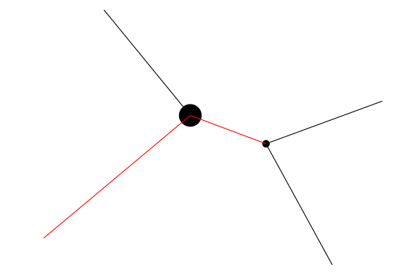
foreach(Pkg.add, ["IJulia", "Ipopt", "Interact", "Reactive", "JuMP", "Compose", "MacroTools"]) 

Consider a simple two-dimensional system, shown schematically in the figure.
Red lines there are marked springs, black - inextensible ropes, a small cup - a weightless block, a large one - a load. The ropes have a length, the spring has a length and rigidity. The variable coordinates are called:

(x, y) - coordinates of the load (large circle)
(xctl, yctl) - coordinates of the “controlling end” of the rope, 1.7 long, tied to the load.
(xp, yp) - coordinates of a weightless point block capable of sliding along the rope.

One spring of length 0.1 and stiffness 1 is fixed at point (0.3) and attached to the load. The second spring with a length of 0.15 and a stiffness of 5 connects the load and the block, which slides along the rope with a length of 6 fixed at the points (5.1) and (4.5.5).

(The parameters were selected evolutionarily, so that I would be clear and understandable how it behaves when adding new features)

  @wire(x,y, xctl,yctl, 1.7) @wire(xp, yp, 5.0,1.0, 4.5,5.0, 6.0) @energy([w(x,y, 0,3, 1, 0.1), w(x,y, xp,yp, 5, 0.15), 0.4*y]) 

The wire macro sets the restriction of “binding an inextensible rope” of a given length to two objects or two objects and a block.

The energy macro describes the minimized energy function - the special term w describes the spring (with a given stiffness and length), and 0.4 * y is the load energy in the gravitational field, which is too simple to come up with a special syntax for it.

These macros are expressed in terms of library NLconstraint and NLobjective (linear constraint and objective are more efficient, but they cannot cope with our functions):

 @NLconstraint(m, (x-xctl)^2+(y-yctl)^2 <= 1.7) @NLconstraint(m, sqrt((5.0-xp)^2+(1.0-yp)^2) + sqrt((4.5-xp)^2+(5.0-yp)^2) <= 6.0) @NLobjective(m, Min, 1*(sqrt(((x-0)^2 + (y - 3)^2)) - 0.1)^2 + 5*(sqrt((x - xp)^2 + (y - yp)^2) - 0.15)^2 + 0.4*y) 

Using less than or equal to "equal to" means that the rope may sag, but not stretch. For two points, you can use strict equality if you need to connect them with a "hard rod", replacing the corresponding macro.


Now we will describe the controls:

 xctl = slider(-2:0.01:5, label="X Control") xctlsig = signal(xctl) yctl = slider(-1:0.01:0.5, label="Y Control") yctlsig = signal(yctl) 

let's connect them to our system:

 ops = map(myModel, xctlsig, yctlsig) 

And display this in notebook:

 @manipulate for xc in xctl, yc in yctl, op in ops compose(context(), # text(150px, 220px, "m = $(op[2]) $(op[3])"), # text(150px, 200px, "p = $(op[4]) $(op[5])"), circle(pscale(op[2], op[3])..., 0.03), circle(pscale(op[4], op[5])..., 0.01), l(op[2], op[3], op[4], op[5], color="red"), l(op[2], op[3], 0, 3, color="red"), l(op[2], op[3], xc, yc), l(op[4], op[5], 5, 1), l(op[4], op[5], 4.5,5) ) end 

An easy way to start a notebook: dial Julia REPL using IJulia notebook() . This should open in the browser " http: // localhost: 8888 / tree ". There you have to select “new” / “Julia”, copy the code in the input field and press Shift-Enter.