Anatomy of KD-Trees

This article is fully devoted to KD-Trees: I describe the subtleties of constructing KD-Trees, the subtleties of implementing the 'near' search functions in the KD-Tree, as well as possible 'pitfalls' that arise in the process of solving certain subtasks of the algorithm. In order not to confuse the reader with terminology (plane, hyper-plane, etc.), and indeed for convenience, it is assumed that the main action takes place in three-dimensional space. However, where necessary, I note that we are working in a space of another dimension. In my opinion, the article will be useful both to programmers and to all those who are interested in learning the algorithms: someone will find something new for themselves, and someone will simply repeat the material and perhaps add comments to the article in the comments. In any case, I ask everyone under the cat.

Introduction

KD-Tree (K-dimensional tree), a special 'geometric' data structure that allows you to split the K-dimensional space into 'smaller parts', by means of a cross section of this very space by hyperplanes ( K> 3 ), planes ( K = 3 ), straight lines ( K = 2 ) well, and in the case of a one-dimensional space-point (performing a search in such a tree, we get something similar to binary search ).
It is logical that such a partition is usually used to narrow the search range in K-dimensional space. For example, searching for a near object (vertex, sphere, triangle, etc.) to a point, projecting points onto a 3D grid, ray tracing (actively used in Ray Tracing), etc. At the same time, space objects are placed in special parallelepipeds - bounding boxes. (A bounding box is a parallelepiped that describes the original set of objects or the object itself if we build a bounding box only for it. For points, the bounding box is taken as the bounding box. box with zero surface area and zero volume), the sides of which are parallel to the coordinate axes.

The process of dividing the node

So, before using the KD-Tree, you need to build it. All objects are placed in one large bounding box, describing the objects of the original set (each object is limited to its bounding box), which is then divided (divided) by a plane parallel to one of its sides into two. Two new nodes are added to the tree. In the same way, each of the parallelepipeds obtained is divided into two, etc. The process is completed either by a special criterion (see SAH ), or when a certain depth of the tree is reached, or when a certain number of elements are reached inside the tree node. Some elements can simultaneously enter both left and right nodes (for example, when triangles are considered as tree elements).

I will illustrate this process with the example of the set of triangles in 2D:
')

Figure 1 shows the original set of triangles. Each triangle is placed in its own bounding box, and the entire set of triangles is inscribed in one large root bounding box.


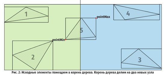
In Fig.2, we divide the root node into two nodes (OX): triangles 1, 2, 5 fall into the left node, and 3, 4, 5 into the right node.


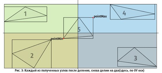
In Figure 3 , the resulting nodes are again divided into two, and triangle 5 is included in each of them. When the process ends, we get 4 leaf nodes.

Of great importance is the choice of the plane to divide the tree node. There are a huge number of ways to do this, I cite only some of the most frequently used methods in practice (it is assumed that the initial objects are placed in one large bounding box, and the separation takes place parallel to one of the coordinate axes):

⦁ Method 1 : Select the largest side of the bounding box. Then the cutting plane will pass through the middle of the selected side.

⦁ Method 2 : Cut by median: we will sort all primitives by one of the coordinates, and by the median we call the element (or center of the element), which is in the middle position in the sorted list. The secant plane will pass through the median so that the number of elements on the left and right will be approximately equal.

⦁ Method 3 : Using the alternation of sides when splitting: at a depth of 0, beat through the middle of the side parallel to OX, the next level is through the middle of the side parallel to OY, then through OZ, etc. If we 'walked through all the axes', then we start the process again. The exit criteria are described above.

⦁ Method 4 : The most 'smart' option is to use the SAH (Surface Area Heuristic) bounding box separation evaluation function. (This will be discussed in detail below). SAH also provides a universal criterion for stopping the division of a node.

Methods 1 and 3 are good when it comes to the speed of building a tree (as it is trivial to find the middle of the side and draw a plane through it, sifting out the elements of the original set 'to the left' and 'to the right'). At the same time, they quite often give an incomplete representation of the partitioning of space, which can negatively affect the basic operations in the KD-Tree (especially when tracking a ray in a tree).

Method 2 allows you to achieve good results, but requires a considerable amount of time that is spent on sorting node elements. Like methods 1, 3, it is quite simple to implement.

Of greatest interest is the method using the 'smart' SAH heuristics (method 4).

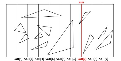
The bounding box of a tree node is divided by N (parallel axes) planes to N + 1 parts (the parts are usually equal) on each side (in fact, the number of planes for each side can be any, but for simplicity and efficiency they take a constant) . Further, at the possible points of intersection of the plane with the bounding box, the value of the special function is calculated: SAH. The division is made by the plane with the smallest value of the SAH function (in the figure below, I assumed that the minimum is reached in SAH [7], therefore, the division will be performed by this plane (although here 2D space is so direct)):



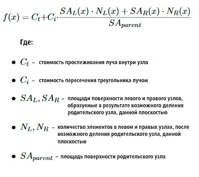
The value of the SAH function for the current plane is calculated as follows:



In my KD-Tree implementation, I divide each side into 33 equal parts using 32 planes. Thus, according to the results of the tests, I managed to find the 'golden' mid-speed of the basic functions of the tree / speed of building the tree.

As SAH heuristics, I use the function shown in the figure above.

It is worth noting that for making a decision, only a minimum of this function is required for all cutting planes. Consequently, using the simplest mathematical properties of inequalities, as well as discarding multiplication by 2 when calculating the surface area of ​​a node (in 3D) ( SAR, SAL, SA ), this formula can be significantly simplified. To the full extent, calculations are made only once per node: when evaluating the criterion for exiting the division function. Such a simple optimization gives a significant increase in the speed of building a tree ( x2.5 ).

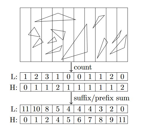
To effectively calculate the value of the SAH function, you must be able to quickly determine how many node elements are to the right of this plane, and how many are to the left. The results will be unsatisfactory if the rough, so-called brute force approach with quadratic asymptotics is used as an algorithm. However, with the use of the 'binned' method, the situation changes significantly for the better. The description of this method is given below:

Suppose that we divide the side of the bounding box into N equal parts (the number of planes- (N-1)), the bounding box is stored by a pair of coordinates (pointMin, pointMax-see. Fig. 1 ), then in one pass through all elements of the node we can accurately determine for each plane how many elements lie to the right and how many to the left of it. Create two arrays of N elements each, and initialize with zeros. Let it be arrays with the names aHigh and aLow . Consistently run through all the elements of the site. For the current element, we check which of the parts pointMin and pointMax of its bounding box falls into. Accordingly, we obtain two indices per set element. Let it be indexes with the names iHigh (for pointMax) and iLow (for pointMin). After that, do the following: aHigh [iHigh] + = 1, aLow [iLow] + = 1.

After going through all the elements, we get the filled arrays aHigh and aLow. For the aHigh array, we calculate the partial-postfix (suffix) sums, and for aLow, we calculate the partial-prefix (prefix) sums (see the figure). It turns out that the number of elements to the right ( and only to the right! ) From the plane with the index i will be equal to aLow [i + 1], the number of elements to the left ( and only to the left! ): AHigh [i], the number of elements that come in as to the left and to the right nodes: AllElements-aLow [i + 1] -aHigh [i].

The problem is solved, and an illustration of this simple process is given below:



I would like to note that obtaining a predetermined number of elements to the left and right of the 'beating' plane allows us to pre-allocate the necessary amount of memory for them (after all, after obtaining the minimum of SAH, we need to go through all the elements once more and place each in the required array , (and the use of banal push_back (if reserve is not called) results in a permanent allocation of memory, a very expensive operation), which has a positive effect on the speed of the tree-building algorithm (x3.3).

Now I would like to describe in more detail the purpose of the constants used in the SAH calculation formula, and also tell about the criteria for stopping the division of this node.

Looking through the constants cI and cT , it is possible to achieve a more dense tree structure (or vice versa), sacrificing the running time of the algorithm. In many articles devoted primarily to building a KD-Tree for a Ray Tracing render, the authors use the values cI = 1., cT = [1; 2] : the greater the value of cT, the faster the tree is built, and the worse the results of ray tracing in such a tree.

In my own implementation, I use the tree to search for 'near', and, paying due attention to the results of testing and searching for the necessary coefficients, it can be noted that high cT values ​​give us nodes that are not densely filled with elements. To avoid this situation, I decided to set the value of cT to 1., and the value of cI to test on different-large data units. As a result, we managed to get a fairly dense tree structure, having paid off with a significant increase in time during construction. This action was reflected positively on the results of the search for “near”; the search speed increased.

The criterion for stopping the division of a node is quite simple:



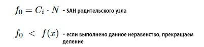
In other words: if the cost of tracking the child nodes is greater than the cost of tracking the parent node, then the division needs to be stopped.

Now that we have learned how to divide a KD-Tree node, I’ll tell you about the initial cases where the number of elements in a node is quite large, and the stopping criteria for the number of elements lead the algorithm to infinity. Actually, all the attention to the picture (for example, triangles in 2D):



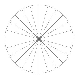
I call such situations "fan-shaped" (they have a common point of contact, coinciding objects, I also attribute to this category). It can be seen that no matter how we perform the cutting plane, the central point somehow falls into one of the nodes, and with it the triangles for which it is common.

Tree building process

We learned how to divide a tree node, now it remains to apply the knowledge gained to the process of building the entire tree. Below I give a description of my implementation of building a KD-Tree.

The tree is built from the root. In each node of the tree, I store pointers to the left and right subtrees, if there is no such node, then it is considered leaf (leaf ie). Each node stores a bounding box that describes the objects of this node. In leaf ( and only in leaf! ) Nodes I store the indices of those objects that are included in this node. However, in the process of building, memory for nodes is allocated in chunks (i.e., immediately for K nodes: firstly, it is more efficient to work with the memory manager, secondly, contracting elements are ideal for caching). Such an approach prohibits storing tree nodes in a vector, because the addition of new elements to a vector can lead to memory allocation for all existing elements to another place.

Accordingly, pointers to subtrees lose all meaning. I use a container of type list (std :: list), each element of which is a vector (std :: vector), with a predetermined size (constant). I build a tree multithreadedly (I use Open MP), that is, each subtree is built in a separate thread (x4 to speed). For copying indexes into a leaf node, use the move semantics (C ++ 11) (+ 10% of the speed) is ideal.

Search 'near' to a point in KD-Tree

So, the tree is built, let's go on to the description of the implementation of the search operation in the KD-Tree.

Suppose that we search in the set of triangles: given a point, it is required to find the nearest triangle to it.

Solving the problem with the use of bruteforce is unprofitable: for a set of N points and M triangles, the assymptotics will be O (N * M). In addition, I would like the algorithm to calculate the distance from the point to the triangle 'honestly' and do it quickly.

Use the KD-Tree and do the following:

⦁ Step 1 . Find the closest leaf node to this point (at each node, as you know, we store the bounding box, and we can safely calculate the distance to the center ((pointMax + pointMin) * 0.5) the bounding box of the node) and denote it by the nearestNode.

⦁ Step 2 . The search method among all elements of the found node (nearestNode). The resulting distance is denoted minDist.

⦁ Step 3 . Construct a sphere with center at the initial point and radius of length minDist. Check whether this sphere is completely inside (that is, without any intersection of the sides of the bounding box-node) nearestNode. If it is, then the near element is found, if not, then go to step 4.

⦁ Step 4 . Run from the root of the tree, search for the near element in the radius: going down the tree, we check whether the right or left nodes intersect (in addition, the node can lie completely inside the sphere or the sphere inside the node ...) this sphere. If a node has been crossed, then we perform a similar check for the internal nodes of the same node. If we come to a leaf node, then we perform an over-search for the neighbor in this node and compare the result with the length of the sphere radius. If the radius of the sphere is greater than the distance found, update the length of the sphere radius with the calculated minimum value. Further descents through the tree occur with the updated length of the sphere radius (if we use a recursive algorithm, then the radius is simply passed to the function by reference, and then, where necessary, updated).

The following figure helps to understand the essence of the algorithm described above:



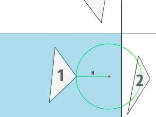
According to the picture : suppose we found the nearest leaf node (blue in the picture) to this point (highlighted in red), then, having performed the search for the nearest leaf in the node, we get that the triangle with ichounks 1 is, however, as you can see, this is not so . A circle with radius R intersects the adjacent node, therefore, the search must be performed in this node, and then compare the newly found minimum with what is already there. As a result, it becomes obvious that the neighbor is a triangle with index 2.

Now I would like to talk about the effective implementation of intermediate operations used in the search algorithm of the "neighbor".

When searching for a neighbor in a node, you must be able to quickly calculate the distance from a point to a triangle. I will describe the simplest algorithm:

We find the projection of the point A (the point to which we are looking for the proximal one) on the plane of the triangle. The found point is denoted by P. If P lies inside the triangle, then the distance from A to the triangle is equal to the length of the segment AP, otherwise we find the distances from A to each of the sides (segments) of the triangle, choose a minimum. Problem solved.

The described algorithm is not the most effective. A more efficient approach relies on the search and analysis (finding the minimum of a gradient, etc.) of a function whose values ​​are all possible distances from a given point to any point in the triangle. The method is rather complicated in perception and, I think, deserves a separate article (for the time being it is implemented in my code, and you will find a link to the code below). You can get acquainted with the method according to [1] . According to the test results, this method turned out to be 10 times faster than what I described earlier.

Determining whether a sphere is centered at point O and radius R inside a specific node represented by a bounding box is simple (3D):

inline bool isSphereInBBox(const SBBox& bBox, const D3& point, const double& radius) { return (bBox.m_minBB[0] < point[0] - radius && bBox.m_maxBB[0] > point[0] + radius && bBox.m_minBB[1] < point[1] - radius && bBox.m_maxBB[1] > point[1] + radius && bBox.m_minBB[2] < point[2] - radius && bBox.m_maxBB[2] > point[2] + radius); } 

With the algorithm for determining the intersection of a sphere with a bounding box of a node, finding a node inside a sphere, or a sphere inside a node, things are somewhat different. I will illustrate again (picture taken from [2]) and give the correct code that allows you to perform this procedure (in 2D, 3D-like):

 bool intersects(CircleType circle, RectType rect) { circleDistance.x = abs(circle.x - rect.x); circleDistance.y = abs(circle.y - rect.y); if (circleDistance.x > (rect.width/2 + circle.r)) { return false; } if (circleDistance.y > (rect.height/2 + circle.r)) { return false; } if (circleDistance.x <= (rect.width/2)) { return true; } if (circleDistance.y <= (rect.height/2)) { return true; } cornerDistance_sq = (circleDistance.x - rect.width/2)^2 + (circleDistance.y - rect.height/2)^2; return (cornerDistance_sq <= (circle.r^2)); } 

First (the first couple of lines) we reduce the calculations of 4 quadrants to one. In the next pair of lines, check if the circle is in the green area. If it lies, then there is no intersection. The next couple of lines will check if the circle is in the orange or gray area of ​​the picture. If included, then the intersection is detected.

Next you need to check whether the circle intersects the corner of the rectangle (this is done by the following lines of code).

Actually, this calculation returns 'false' for all circles whose center is within the red area, and 'true' for all circles whose center is in the white area.

In general, this code provides what we need (I provided the implementation of the code for 2D here, but in my KD-Tree code I use the 3D version).

It remains to talk about the speed of the search algorithm, as well as critical situations that slow down the search in KD-Tree.

As mentioned above, the 'fan' situations generate a large number of elements inside the node, the more they are, the slower the search. Moreover, if all elements are equidistant from the given point, then the search will be carried out behind O (N) (the set of points that lie on the surface of the sphere, and the nearest one is searched to the center of the sphere). However, if these situations are removed, then an average search will be equivalent to descending a tree with enumerating elements in several nodes, i.e. for O (log (N)) . It is clear that the speed of the search depends on the number of visited leaf nodes of the tree.

Consider the following two figures:

The essence of these figures is that if the point to which we are looking for the near element is very, very far from the original bounding box of the set, then a sphere with a radis of length minDist (distance to the near) will cross many more nodes than if we looked at the same sphere, but with a center at a point much closer to the original bounding box of the set (of course, minDist changes). In general, the search for the nearest to a highly distant point is slower than the search for a point close to the original set. My tests confirmed this information.

Results and summation

As a summary, I would like to add a few words about my KD-Tree implementation and give the results. Actually, the code design was developed so that it could be easily adapted to any objects of the original set (triangles, spheres, points, etc.). All you need is to create a class inheritor, with overridden virtual functions. Moreover, my implementation also provides for the transfer of a special class Splitter , user-defined. This class, or rather its virtual split method, determines where exactly the cutting plane will pass. In my implementation, I provide a SAH-based decision making class. Here, I will note that in many articles devoted to accelerating the construction of a KD-Tree based on SAH, many authors use the simplest techniques for searching for a cutting plane (like dividing by center or median) for initial depths of a tree (generally, when the number of elements in a tree node is large). ), and SAH heuristics are used only at the moment when the number of elements in a node is small.

My implementation does not contain such tweaks, but allows you to quickly add them (you just need to expand the KD-Tree constructor with a new parameter and call the member function of the construction with the necessary splitter, controlling the necessary restrictions). Search in a tree I carry out multi-threaded. I make all calculations in numbers with double precision ( double ). The maximum depth of a tree is set by a constant (by default-32). Some #defines are defined that allow, for example, to traverse the tree when searching without recursion (with recursion, though the output is faster — all nodes are elements of a certain vector (that is, they are located next to each other in memory), which means they are well cached). Together with the code, I provide test datasets (3D models of the 'changed format OFF' with different numbers of triangles inside (from 2 to 3,000,000)). The user can dump the constructed tree (DXF format) and view it in the corresponding graphical program. The program also logs (you can turn on / off) the quality of building a tree: the tree depth is reset, the maximum number of elements in a leaf node, the average number of elements in leaf nodes, the operation time . In no case do I claim that the resulting implementation is perfect, but what’s really there, I myself know the places where I missed (for example, I don’t pass the allocator to the template parameter, the frequent presence of the C code (I do not read and write files using streams) , unnoticed bugs, etc. are possible — it's time to fix it). And of course, the tree is made and optimized strictly for working in 3D space.

I tested the code on a laptop with the following characteristics: Intel Core I7-4750HQ, 4 core (8 threads) 2 GHz, RAM-8gb, Win x64 app on Windows 10 . I took the following coefficients for calculating SAH: cT = 1., cI = 1.5 . And, if we talk about the results, it turned out that at 1, 5 million. triangles tree is built in less than 1.5 seconds. At 3 million in 2.4 seconds. For 1.5 million points and 1.5 million triangles (the points are located not very far from the original model), the search was completed in 0.23 seconds, and if the points are removed from the model, the time increases, up to 3 seconds. For 3 million points (again, close to the model) and 3 million triangles, the search takes about 0.7 seconds. I hope nothing is confused. Finally, an illustration of the visualization of the constructed KD-Tree:

useful links

[0] : My KD-Tree implementation on GitHub
[1] : Search for distance from point to triangle
[2] : Definitions of intersections of a circle and a rectangle
[3] : KD-Tree Description on Wikipedia
[4] : Interesting SAH article
[5] : Description KD-Tree on ray-tracing.ru