As a programmer, I bought a car. Part II
In the previous article, on the example of buying a Mercedes-Benz E-klasse not older than the 2010 release worth up to 1.5 million rubles in Moscow, the task of finding profitable cars was considered. Under the best you should understand the proposals, the price of which is below the market at the moment among the ads collected from all the most reputable sites for the sale of used cars in the Russian Federation.
At the first stage, the multiple linear regression was chosen as the machine learning method, the legitimacy of its use, as well as the pros and cons were considered. A simple linear regression was chosen as an evaluation algorithm. Obviously, there are still many machine learning methods for solving the set regression problem. In this article I would like to tell you exactly how I chose the most optimal machine learning algorithm for the studied model, which is currently used in the service I have implemented - robasta.ru .

Applicants for the title of "champion":
')
Before making a choice, all the above algorithms were investigated, so I wanted to tell you in detail about each of them. However, this way of searching “head on” is not quite optimal, it is wiser to first conduct additional research on the task.
In addition to the Mercedes-Benz E-klasse, I was impressed by the Audi A5, especially with a 239 hp diesel engine, which has good dynamics (6 seconds to 100 km / h) and a reasonable tax. Looking at the dependence of prices on the engine power of this creation of German engineers (visualization below), many questions disappear by themselves.
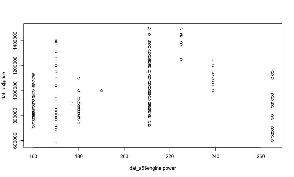
There can be no talk of linear dependence here, so the algorithms based on the linear dependence of the explained variable (cost, in our case) on the regressors can be safely discarded. The use of polynomial and non-linear models is illegal for the reason that the type of dependence of one or another regressor on the price for each individual car model is unknown in advance.
Thus, taking the above considerations into account, we can only consider algorithms based on decision trees - Random forest and Xgboost (with two types of boosting - xgbDart, xgbTree), and choose the optimal one.
It should be noted that the optimal algorithm is the one that will show itself best (min RMSE ) for cross-validation and delayed selection.
Before proceeding to the “blind” application of the selected algorithms, in the next chapter I would like to highlight in more detail the question of their settings.
Cross-validation (V) is often used to evaluate the real capabilities of the model and adjust its parameters in machine learning tasks. There is a set of partitions of the initial sample into the training and control subsamples. For each of the breaks, the algorithm is adjusted by the training subsample, then its control error is estimated at the control.
The estimate of the cross-check is the average over all partitions of the error on the control subsamples.
For an unbiased estimate of the probability of error obtained through cross-validation, it is necessary that the training and control samples form a non-intersecting subset, in order to avoid the phenomenon of overtraining .
Cross-check variations:
Each of the above cross-validation methods can be characterized using bias and variance. The offset characterizes the accuracy of the estimate. Dispersion characterizes the accuracy (precision) assessment.
In general, the offset of the cross-validation method depends on the size of the validation sample. If the size of the validation sample is 50% of the source data (2-block cross-validation), the final estimate of the standard deviation will be more biased than in the case when this size is 10% of the source data. On the other hand, a smaller size of the validation sample increases the variance, since each validation sample contains less data to obtain a stable MSE value.
Thus, when it comes to k-block cross-validation, then to minimize displacement, choose the maximum k, and to reduce variance, use the multiple k-block method that does this task better than once.
As for the MCMB, for this type of cross-validation, the size of the validation sample has a slightly larger effect on the variance than the number of repetitions of the process. It should also be noted that the number of repetitions of the process does not have a significant effect on the displacement.
Thus, for the MCMC method, it is recommended to use a validation sample of small size (for example, 10%) and perform a large number of repetitions to reduce the variance.
However, other things being equal, the use of multiple 10-block HF provides less variance, which is primarily due to the fact that, for this method, the same data element cannot be found in different samples, unlike the MCMB.
At the end of our reasoning, I would like to make a reservation that with large amounts of data a 10-block or even 5-block single KV gives quite acceptable results, in our task, we will use a multiple 10-block cross-check to adjust the model.
“Random Forest” is an algorithm that randomly creates a set of decision trees for the received data and then averages the results of their predictions. The tree building algorithm is very fast, so it’s not hard to make as many trees as you need.
From a practical point of view, the method described above has one huge advantage: it almost does not require configuration. If we take any other machine learning algorithm, be it a regression or a neural network, they all have a lot of parameters, and we should be able to choose them for a specific task. RF, in fact, has only one important parameter that requires adjustment - mtry (the size of a random subset selected at each step of building the tree). However, even using the default value, you can get very acceptable results.
As in the previous article , we replace the missing values (N / A) with the median values for all regressors, exclude the engine size from the sample (due to the strong correlation of the parameter with the power) and look at the capabilities of this algorithm.
For cross-validation, we will use the caret package, which is more capable of assessing the quality of the model than rfcv .
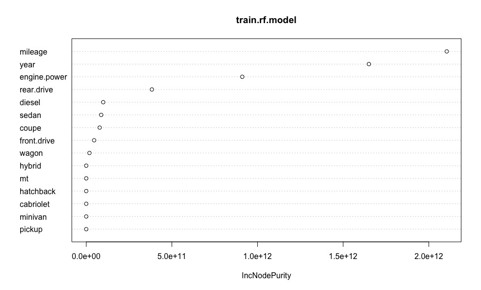
Let us construct a graph visually illustrating the importance of each of the predictors of the model.
The obtained average error in estimating the cost of a car is equivalent to the same value obtained for linear regression. Let me remind you that when building a linear model, unlike RF, we got rid of emissions , which led to additional inaccuracies in the estimates of the cost of cars. Thus, it can be argued about the robustness of the “random forest” to emissions.
The idea of gradient boosting is to build an ensemble of elementary models sequentially refining each other. Each subsequent elementary model is trained on the “mistakes” of the ensemble from the previous elementary models, the model responses are weightedly summed up.
“Busch” can be used for almost any model — general linear, generalized linear, decision trees, K-nearest neighbors, and many others.
The features of the implementation of the algorithm of boosting in xgboost can be attributed, firstly, the use of the second derivative of the loss function in addition to the first, which increases the efficiency of the algorithm. Secondly, the presence of built-in regularization , which helps to fight retraining . Finally, the ability to define custom loss functions and quality metrics.
Thanks to the experimental parameter num_parallel_tree, you can set the number of trees that are simultaneously created and present Random Forest as a special case of a booster model with one iteration. And if you use more than one iteration, you will get the boosting of “random forests”, when each “random forest” acts as an elementary model.
In this article, we will consider only one type of boosting - xgbTree, since xgbDart gives similar results.
We construct a graph demonstrating the importance of each of the predictors of the model.

XGboost for this particular case showed slightly more accurate estimates of the value of cars. It is a matter of concern for a large number of hyperparameters that require reconfiguration depending on the brand and model of car chosen. In this regard, for use on the robasta.ru service , preference was given to the Random Forest algorithm.
Now, when the choice of "champion" is over, it's time to look at him in action.
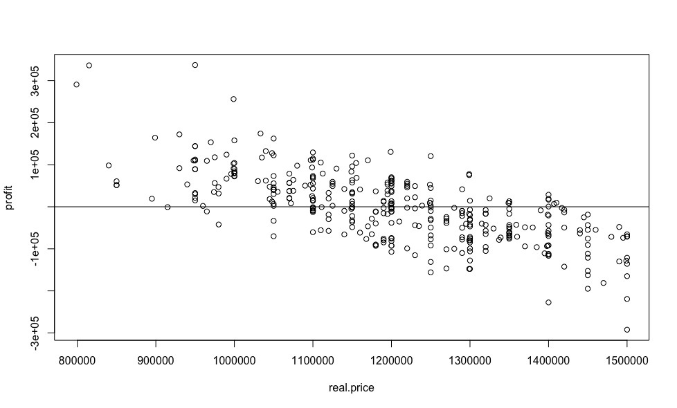
As for the linear regression in the previous article , we construct a graph of the dependence of the benefits on the price.
And now we will calculate the benefit as a percentage.
The results obtained are very weakly similar to the results obtained using linear regression, and look more plausible, despite the almost identical RMS for both models.
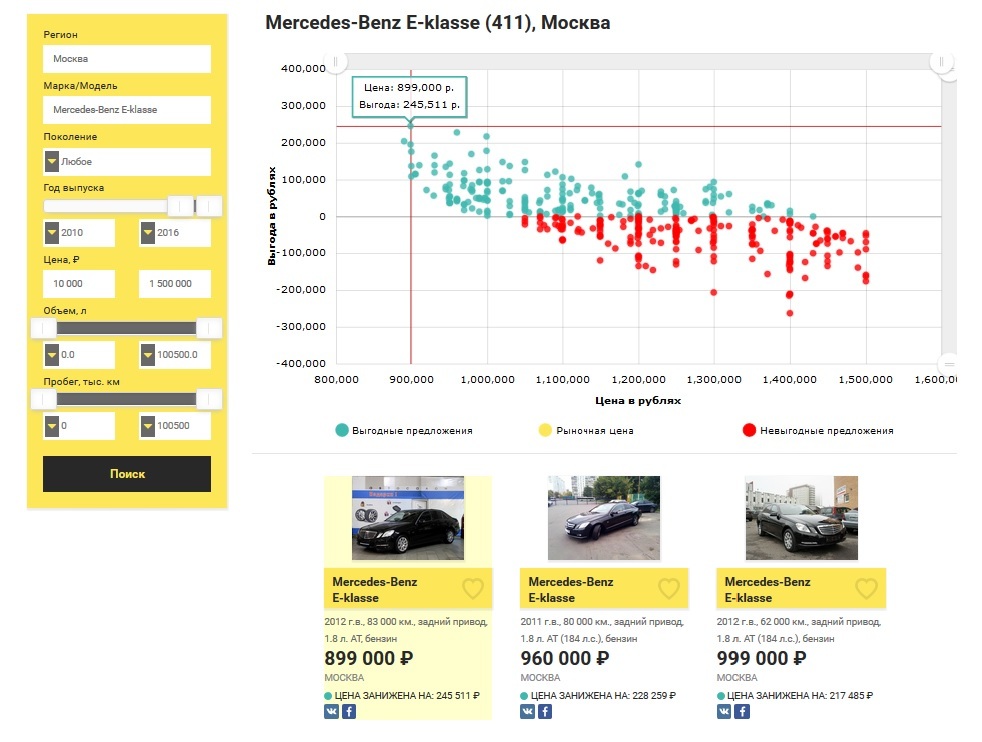
To compare the results in this article, we used a sample from the last publication , so let's see how many lucrative offers of a Mercedes-Benz E-klasse are not older than the 2010 release, worth up to 1.5 million rubles in Moscow on the market now.
Summarizing all the above, I can say with confidence that for the selection of used cars we got a powerful tool that is not sensitive to “fake” ads, working in real time. You no longer need to sit for hours on several sites with advertisements for the sale of cars and drive to watch potentially unprofitable offers.
But that's not all, now, using the considered mathematical apparatus, Robasta can help not only those who want to buy, but also those who want to sell their car.
When selling your car, of course, you want to at least not be cheap and sell it in a short time. For a quick and profitable sale of your car you need to understand the contribution of various characteristics in its value.
To solve this problem, on the basis of the same “random forest”, a service was developed to evaluate the car . You fill in all the fields of the search form, in accordance with the parameters of your car, after which the model is trained on the basis of market offers at the moment. If there are five or more ads on the market, the algorithm for the data you have filled out predicts the price and provides several interesting features depending on the overall picture of the market. It is worth emphasizing that in order to achieve the greatest accuracy, only cars of the same generation as yours are selected for analysis. The results of the evaluation of your car are generated in the form of a pdf report , the cost of which is 99 ₽.

Currently, various areas for further development are being worked out, among which the following can be called the main ones:
Relatively new cars (mileage up to 100 thousand km) are often sold before large expensive MOT, these data are useful to take into account in the model. Therefore, now I am in search of reliable partners among medium and large car dealers.
The opening of an offline center for the selection and evaluation of cars in Moscow, which, thanks to the implemented algorithm, will be much less expensive than its competitors.
Creating a convenient API for providing functionality to “intellectual resellers”.
Do you want something to help in the implementation of the tasks I voiced or to offer your ideas? Write, I am always ready to consider any kind of cooperation.
At the first stage, the multiple linear regression was chosen as the machine learning method, the legitimacy of its use, as well as the pros and cons were considered. A simple linear regression was chosen as an evaluation algorithm. Obviously, there are still many machine learning methods for solving the set regression problem. In this article I would like to tell you exactly how I chose the most optimal machine learning algorithm for the studied model, which is currently used in the service I have implemented - robasta.ru .
Algorithm selection
Applicants for the title of "champion":
')
- Multiple linear (simple) regression
- Lasso regression
- Ridge regression
- Robust regression
- Vowpal wabbit
- Polynomial and nonlinear regression
- Random forest
- Xgboost
Before making a choice, all the above algorithms were investigated, so I wanted to tell you in detail about each of them. However, this way of searching “head on” is not quite optimal, it is wiser to first conduct additional research on the task.
In addition to the Mercedes-Benz E-klasse, I was impressed by the Audi A5, especially with a 239 hp diesel engine, which has good dynamics (6 seconds to 100 km / h) and a reasonable tax. Looking at the dependence of prices on the engine power of this creation of German engineers (visualization below), many questions disappear by themselves.
There can be no talk of linear dependence here, so the algorithms based on the linear dependence of the explained variable (cost, in our case) on the regressors can be safely discarded. The use of polynomial and non-linear models is illegal for the reason that the type of dependence of one or another regressor on the price for each individual car model is unknown in advance.
Thus, taking the above considerations into account, we can only consider algorithms based on decision trees - Random forest and Xgboost (with two types of boosting - xgbDart, xgbTree), and choose the optimal one.
It should be noted that the optimal algorithm is the one that will show itself best (min RMSE ) for cross-validation and delayed selection.
Before proceeding to the “blind” application of the selected algorithms, in the next chapter I would like to highlight in more detail the question of their settings.
Cross-validation
Cross-validation (V) is often used to evaluate the real capabilities of the model and adjust its parameters in machine learning tasks. There is a set of partitions of the initial sample into the training and control subsamples. For each of the breaks, the algorithm is adjusted by the training subsample, then its control error is estimated at the control.
The estimate of the cross-check is the average over all partitions of the error on the control subsamples.
For an unbiased estimate of the probability of error obtained through cross-validation, it is necessary that the training and control samples form a non-intersecting subset, in order to avoid the phenomenon of overtraining .
Cross-check variations:
- k-block cross-validation (k-fold cross-validation).Read moreThis method randomly splits data into k non-overlapping blocks of approximately the same size. Alternately, each block is treated as a validation sample, and the remaining k-1 blocks are treated as a training sample. The model is trained in k-1 blocks and predicts a validation block. The model's forecast is estimated using the selected indicator: accuracy (accuracy), standard deviation (RMSE), etc. The process is repeated k times, and we get k estimates for which the average value is calculated, which is the final estimate of the model. Usually k is chosen equal to 10, sometimes 5. If k is equal to the number of elements in the original data set, this method is called cross-validation on individual elements (this article is not considered).
- Multiple k-block cross-validation (repeated k-fold cross-validation).Read moreIn this method, k-block cross-validation is performed several times. For example, a 5-fold 10-block cross-validation will give 50 estimates, on the basis of which the average estimate will then be calculated. Note that this is not the same as 50-block cross-validation.
- Monte-Carlo-based cross validation (PEC, Monte Carlo cross-validation, leave-group-out cross-validation).Read moreThis method randomly splits the initial data set into a training and validation sample in a given proportion in a specified number of times.
Each of the above cross-validation methods can be characterized using bias and variance. The offset characterizes the accuracy of the estimate. Dispersion characterizes the accuracy (precision) assessment.
In general, the offset of the cross-validation method depends on the size of the validation sample. If the size of the validation sample is 50% of the source data (2-block cross-validation), the final estimate of the standard deviation will be more biased than in the case when this size is 10% of the source data. On the other hand, a smaller size of the validation sample increases the variance, since each validation sample contains less data to obtain a stable MSE value.
Thus, when it comes to k-block cross-validation, then to minimize displacement, choose the maximum k, and to reduce variance, use the multiple k-block method that does this task better than once.
As for the MCMB, for this type of cross-validation, the size of the validation sample has a slightly larger effect on the variance than the number of repetitions of the process. It should also be noted that the number of repetitions of the process does not have a significant effect on the displacement.
Thus, for the MCMC method, it is recommended to use a validation sample of small size (for example, 10%) and perform a large number of repetitions to reduce the variance.
However, other things being equal, the use of multiple 10-block HF provides less variance, which is primarily due to the fact that, for this method, the same data element cannot be found in different samples, unlike the MCMB.
At the end of our reasoning, I would like to make a reservation that with large amounts of data a 10-block or even 5-block single KV gives quite acceptable results, in our task, we will use a multiple 10-block cross-check to adjust the model.
Random forest
“Random Forest” is an algorithm that randomly creates a set of decision trees for the received data and then averages the results of their predictions. The tree building algorithm is very fast, so it’s not hard to make as many trees as you need.
From a practical point of view, the method described above has one huge advantage: it almost does not require configuration. If we take any other machine learning algorithm, be it a regression or a neural network, they all have a lot of parameters, and we should be able to choose them for a specific task. RF, in fact, has only one important parameter that requires adjustment - mtry (the size of a random subset selected at each step of building the tree). However, even using the default value, you can get very acceptable results.
As in the previous article , we replace the missing values (N / A) with the median values for all regressors, exclude the engine size from the sample (due to the strong correlation of the parameter with the power) and look at the capabilities of this algorithm.
dat <- read.csv("dataset.txt") # R dat$mileage[is.na(dat$mileage)] <- median(na.omit(dat$mileage)) # NA dat <- dat[-c(1,11)] # set.seed(1) # ( ) split <- runif(dim(dat)[1]) > 0.2 # train <- dat[split,] # (cross-validation) test <- dat[!split,] # (hold-out) For cross-validation, we will use the caret package, which is more capable of assessing the quality of the model than rfcv .
library(caret) # caret fit.control <- trainControl(method = "repeatedcv", number = 10, repeats = 10) train.rf.model <- train(price~., data=train, method="rf", trControl=fit.control , metric = "RMSE") # 10- 10- - train.rf.model # - Read more
Random forest
292 samples
15 predictor
No pre-processing
Resampling: Cross-Validated (10 fold, repeated 10 times)
Summary of sample sizes: 262, 262, 262, 263, 263, 263, ...
Resampling results across tuning parameters:
mtry RMSE Rsquared
2 134565.8 0.4318963
8 117451.8 0.4378768
15 122897.6 0.3956822
RMSE was used for the smallest value.
The final value is used.
library(randomForest) # random forest train.rf.model <- randomForest(price ~ ., train,mtry=8) # - Let us construct a graph visually illustrating the importance of each of the predictors of the model.
varImpPlot(train.rf.model) # rf.model.predictions <- predict(train.rf.model, test) # print(sqrt(sum((as.vector(rf.model.predictions - test$price))^2)/length(rf.model.predictions))) # ( ) [1] 121760.5 The obtained average error in estimating the cost of a car is equivalent to the same value obtained for linear regression. Let me remind you that when building a linear model, unlike RF, we got rid of emissions , which led to additional inaccuracies in the estimates of the cost of cars. Thus, it can be argued about the robustness of the “random forest” to emissions.
Xgboost
The idea of gradient boosting is to build an ensemble of elementary models sequentially refining each other. Each subsequent elementary model is trained on the “mistakes” of the ensemble from the previous elementary models, the model responses are weightedly summed up.
“Busch” can be used for almost any model — general linear, generalized linear, decision trees, K-nearest neighbors, and many others.
The features of the implementation of the algorithm of boosting in xgboost can be attributed, firstly, the use of the second derivative of the loss function in addition to the first, which increases the efficiency of the algorithm. Secondly, the presence of built-in regularization , which helps to fight retraining . Finally, the ability to define custom loss functions and quality metrics.
Thanks to the experimental parameter num_parallel_tree, you can set the number of trees that are simultaneously created and present Random Forest as a special case of a booster model with one iteration. And if you use more than one iteration, you will get the boosting of “random forests”, when each “random forest” acts as an elementary model.
In this article, we will consider only one type of boosting - xgbTree, since xgbDart gives similar results.
fit.control <- trainControl(method = "repeatedcv", number = 10, repeats = 10) train.xgb.model <- train(price ~., data = train, method = "xgbTree", trControl = fit.control, metric = "RMSE") # 10- 10- - train.xgb.model # - Read more
eXtreme Gradient Boosting
292 samples
15 predictor
No pre-processing
Resampling: Cross-Validated (10 fold, repeated 10 times)
Summary of sample sizes: 263, 262, 262, 263, 264, 263, ...
Resampling results across tuning parameters:
eta max_depth colsample_bytree nrounds RMSE Rsquared
0.3 1 0.6 50 114131.1 0.4705512
0.3 1 0.6 100 113639.6 0.4745488
0.3 1 0.6 150 113821.3 0.4734121
0.3 1 0.8 50 114234.6 0.4694687
0.3 1 0.8 100 113960.5 0.4712563
0.3 1 0.8 150 114337.1 0.4685121
0.3 2 0.6 50 115364.6 0.4604643
0.3 2 0.6 100 117576.4 0.4472452
0.3 2 0.6 150 119443.6 0.4358365
0.3 2 0.8 50 116560.3 0.4494750
0.3 2 0.8 100 119054.2 0.4350078
0.3 2 0.8 150 121035.4 0.4222440
0.3 3 0.6 50 117883.2 0.4422659
0.3 3 0.6 100 121916.7 0.4162103
0.3 3 0.6 150 125206.7 0.3968248
0.3 3 0.8 50 119331.3 0.4296062
0.3 3 0.8 100 124385.7 0.3987044
0.3 3 0.8 150 128396.6 0.3753334
0.4 1 0.6 50 113771.6 0.4727520
0.4 1 0.6 100 113951.6 0.4717968
0.4 1 0.6 150 114135.0 0.4710503
0.4 1 0.8 50 114055.0 0.4700165
0.4 1 0.8 100 114345.5 0.4680938
0.4 1 0.8 150 114715.8 0.4655844
0.4 2 0.6 50 116982.1 0.4499777
0.4 2 0.6 100 119511.9 0.4347406
0.4 2 0.6 150 122337.9 0.4163611
0.4 2 0.8 50 118384.6 0.4379478
0.4 2 0.8 100 121302.6 0.4201654
0.4 2 0.8 150 124283.7 0.4015380
0.4 3 0.6 50 118843.2 0.4356722
0.4 3 0.6 100 124315.3 0.4017282
0.4 3 0.6 150 128263.0 0.3796033
0.4 3 0.8 50 122043.1 0.4135415
0.4 3 0.8 100 128164.0 0.3782641
0.4 3 0.8 150 132538.2 0.3567702
Tuning parameter 'gamma' was held constant at a value of 0
Tuning parameter 'min_child_weight' was held constant at a value of 1
RMSE was used for the smallest value.
The final values used for the model were nrounds = 100, max_depth = 1, eta = 0.3, gamma = 0, colsample_bytree = 0.6 and min_child_weight = 1.
library(xgboost) # xgboost xgb_train <- xgb.DMatrix(as.matrix(train[-c(1)] ), label=train$price) # xgb_test <- xgb.DMatrix(as.matrix(test[-c(1)]), label=test$price) # xgb.param <- list(booster = "gbtree", max.depth = 1, eta = 0.3, gamma = 0, subsample = 0.5, colsample_bytree = 0.6, min_child_weight = 1, eval_metric = "rmse") train.xgb.model <- xgb.train(data = xgb_train, nrounds = 100, params = xgb.param) # - We construct a graph demonstrating the importance of each of the predictors of the model.
importance.frame <- xgb.importance(colnames(train[-c(1)]), model = train.xgb.model) # library(Ckmeans.1d.dp) # xgb.plot xgb.plot.importance(importance.frame) xgb.model.predictions <- predict(train.xgb.model, xgb_test) # print(sqrt(sum((as.vector(xgb.model.predictions - test$price))^2)/length(xgb.model.predictions))) # ( ) [1] 118742.8 XGboost for this particular case showed slightly more accurate estimates of the value of cars. It is a matter of concern for a large number of hyperparameters that require reconfiguration depending on the brand and model of car chosen. In this regard, for use on the robasta.ru service , preference was given to the Random Forest algorithm.
Approbation of the selected algorithm
Now, when the choice of "champion" is over, it's time to look at him in action.
library(randomForest) # random forest rf.model <- randomForest(price ~ ., dat,mtry=8) # - predicted.price <- predict(rf.model, dat) # real.price <- dat$price # profit <- predicted.price - real.price # As for the linear regression in the previous article , we construct a graph of the dependence of the benefits on the price.
plot(real.price,profit) abline(0,0) And now we will calculate the benefit as a percentage.
sorted <- sort(predicted.price /real.price, decreasing = TRUE) sorted[1:10] 69 42 122 15 168 248 346 109 231 244 1.412597 1.363876 1.354881 1.256323 1.185104 1.182895 1.168575 1.158208 1.157928 1.154557 The results obtained are very weakly similar to the results obtained using linear regression, and look more plausible, despite the almost identical RMS for both models.
To compare the results in this article, we used a sample from the last publication , so let's see how many lucrative offers of a Mercedes-Benz E-klasse are not older than the 2010 release, worth up to 1.5 million rubles in Moscow on the market now.
Summarizing all the above, I can say with confidence that for the selection of used cars we got a powerful tool that is not sensitive to “fake” ads, working in real time. You no longer need to sit for hours on several sites with advertisements for the sale of cars and drive to watch potentially unprofitable offers.
But that's not all, now, using the considered mathematical apparatus, Robasta can help not only those who want to buy, but also those who want to sell their car.
Car sales
When selling your car, of course, you want to at least not be cheap and sell it in a short time. For a quick and profitable sale of your car you need to understand the contribution of various characteristics in its value.
To solve this problem, on the basis of the same “random forest”, a service was developed to evaluate the car . You fill in all the fields of the search form, in accordance with the parameters of your car, after which the model is trained on the basis of market offers at the moment. If there are five or more ads on the market, the algorithm for the data you have filled out predicts the price and provides several interesting features depending on the overall picture of the market. It is worth emphasizing that in order to achieve the greatest accuracy, only cars of the same generation as yours are selected for analysis. The results of the evaluation of your car are generated in the form of a pdf report , the cost of which is 99 ₽.
At last
Currently, various areas for further development are being worked out, among which the following can be called the main ones:
Relatively new cars (mileage up to 100 thousand km) are often sold before large expensive MOT, these data are useful to take into account in the model. Therefore, now I am in search of reliable partners among medium and large car dealers.
The opening of an offline center for the selection and evaluation of cars in Moscow, which, thanks to the implemented algorithm, will be much less expensive than its competitors.
Creating a convenient API for providing functionality to “intellectual resellers”.
Do you want something to help in the implementation of the tasks I voiced or to offer your ideas? Write, I am always ready to consider any kind of cooperation.
Links
Source: https://habr.com/ru/post/312842/
All Articles