Introduction The classical factor analysis [1] allows, on the basis of a sample of various indicators, to form factor indicators with the required accuracy describing the original object and reducing the dimensionality of the problem by moving to them. Factor indicators are a linear combination of inputs. Thus, factor models are linear.

The neural network allows you to approximate the mapping between the source and target indicators. Moreover, approximable mappings can be nonlinear. A two-layer perceptron allows one to approximate any Boolean function of Boolean variables [2]. A two-level neural network can approximate any continuous function in a uniform metric with any given error ε > 0 , and in the mean square metric, any measurable function defined on a bounded set [3, 4, 5, 6].

To restore the regularities between the parameters, a special neural network learning algorithm is used: the back error propagation algorithm [7]. From the mathematical point of view, this algorithm is a gradient optimization method.

The essence of this method for constructing factor models is that a mathematical model of a neural network with a linear transfer function is used to identify patterns between the parameters. The values ​​of the factor variables are determined to be equal to the values ​​of the output signals of the neurons of the hidden layer of the neural network. Thus, the neural network performs classical factor analysis, i.e. builds linear combinations of source parameters [8, 9, 10].

This paper proposes an improved algorithm for backpropagating an error by introducing an additional term to the error function to construct an interpretable factor structure and solve the problem of factor rotation based on a neural network.

Mathematical model of a neuron. The state of the neuron is described by a set of variables:

input weights where m is the number of input signals ;

free member in the calculation of the output signal. The signal at the output of the neuron is calculated by the formula:

where - the weighted sum of the signals at the inputs of the neuron,

σ is the transfer function of the neuron, for example, sigmoidal function .

Neural network. Separate neurons are combined into layers. The output signals of neurons from one layer arrive at the input to the neurons of the next layer, the model of the so-called multilayer perceptron (Fig. 1). In the software implementation of the author's neural network, the concept of descendant neurons and ancestor neurons is introduced. All neurons that have an input signal from a given neuron are its descendants or passive neurons or axons. All neurons forming the input signals of a given neuron are its ancestors or active neurons or dendrites.

Fig. 1 . Simple neural network (input neurons, hidden neurons, output neuron).

Error propagation algorithm. The back-propagation error algorithm for training a neural network corresponds to minimizing the error function E ( w _ij ) . As such an error function, the sum of squared deviations of the network output signals from the required ones can be used:

,

Where - the output value of the i- th neuron of the output layer,

- the required value of the i- th neuron of the output layer.

In this algorithm, the learning iteration consists of three procedures:

1. The propagation of the signal and the calculation of the signals at the output of each neuron.

   
   

2. Error calculation for each neuron.

   
   

3. Changing the weights of connections.

   
   

By repeatedly cycling the sets of signals at the input and output and back propagation of an error, the neural network is trained. For a multilayer perceptron and a certain type of neuron transfer function, the convergence of this method was proved for a certain type of error function [11].

Calculation of errors. If the transfer function of neurons is sigmoidal, then the errors for neurons of different layers are calculated using the following formulas.

Error calculations for neurons of the output layer are made according to the formula:

,

Where - the desired value at the output of the jth neuron of the output layer L ,

- the signal at the output of the j- th neuron of the output layer L ,

L is the depth of the neural network,

Errors for the neurons of the remaining layers are calculated by the formula:

,

where i - indices of neurons, the descendants of the neuron,

- the signal at the output of the j- th neuron layer l ,

- the connection between the j- th neuron of the l- th layer and the i- th neuron of the ( l +1) -th layer.

Changing the threshold levels of neurons and weights of connections. To change the link weights, use the following formula:

,

,

,

where i is the index of the active neuron (neuron of the source of input signals of passive neurons),

j - passive neuron index,

n is the number of the learning iteration,

α is the coefficient of inertia for smoothing sharp jumps when moving along the surface of the objective function,

0 < η <1 is the multiplier setting the speed of "movement".

Method of building a factor model. Factor analysis is based on the following linear model linking the original indicators and factors :

m is the number of variables

g - the number of factors

- source variables

- common factors

- specific factors.

In the matrix form, the linear model of factor analysis is written in the form:

,

Where - dimension matrix values ​​of m parameters for n objects,

- dimension matrix the values ​​of g factors for n objects,

- dimension matrix values ​​of m specific factors for n objects,

- matrix of factorial dimension display weights,

- diagonal dimension matrix weighting factors specific factors.

In this method of building a factor model, the latent characteristics are assigned to the neurons of the hidden layer. At the same time, the number of neurons in the hidden layer is assumed to be smaller than the number of neurons in the input layer for the implementation of factor compression of the input information. To estimate the number of neurons in the hidden layer, you can apply the Kaiser rule of classical factor analysis. The neurons of the input and output layer are assigned the initial characteristics of the objects of study. When the transfer function of neurons is linear, this configuration of the neural network corresponds to the classical factor analysis (Fig. 2).

Fig. 2 Scheme of the neural network of classical factor analysis (the number of neurons in the input layer is equal to the number of neurons in the output layer, the number of neurons in the hidden layer is less than the number of neurons in the input layer).

Using neural network training, weights of input connections of neurons of the hidden and output layer are calculated, which correspond to the elements of the inverse and direct factor display . Weights of neurons are searched in the interval [-1, 1]. The filling of factors with the initial variables is determined using the values ​​of the elements of the factorial display and the selected threshold level of significance. . The variable i enters the factor j if .

To reveal the relationship between the factor model and the neural network, we use the formulas for obtaining the output signal of the neurons of the hidden layer.

Denote the output of the jth neuron of the hidden layer . The output signal of the i- th neuron of the input layer is denoted by . As a transfer function, we will use a linear function. .

As a result

,

where m is the number of neurons in the input layer;

- the connection between the i- th neuron of the s- th layer and the j- th neuron of the t -th layer,

- threshold level of the i -th neuron of the s -th layer.

Similarly for the output layer:

,

Where - the output value of the i- th neuron of the output layer,

g is the number of neurons in the hidden layer.

The resulting linear relationship of variables corresponds to the classical model of factor analysis, in which factors are linear combinations of source variables. The task of finding factor mappings and factor values ​​is reduced to the task of finding weights of connections and threshold levels of a neural network. Since the factor mapping and factor values ​​are unknown, a network with an intermediate layer is required. The network as a whole performs the identical transformation, i.e. the output signal on the i- th neuron of the input layer is equal to the output signal of the i -th neuron of the output layer. Separate parts of the network (input and output parts) correspond to direct and inverse factor mapping.

Theorem .

Let be and - the weight of the input signals of the output and hidden layer of the neural network with a linear transfer function. The number of neurons on the output layer is equal to the number of neurons in the input layer. A neural network consists of an input, hidden and output layer and performs the same transformation for any input signal (the vector of input signals of the network is equal to the vector of output signals).

Then the following equality holds :

,

Where - the connection between the i - th neuron of the s - th layer and the j - th neuron of the t - th layer ,

g is the number of neurons in the hidden layer.

Proof :

Denote - the output signal of the i- th neuron of the k -th layer,

- i -th output signal of neurons of the first layer.

To search for neural network weights, the following condition must be met:

, the output signal on the i- th neuron of the input layer is equal to the output signal of the i -th neuron of the output layer. From this condition follows an auxiliary condition:

, the change in the i- th input network signal is equal to the change in the i- th output signal. The following equalities are true:

,

where and - input and output signal to change,

.

Suppose that only the i -th input signal was changed .

From these conditions follows:

;

Insofar as then must be performed for all i , since the choice of the i- th input signal was arbitrary.

The theorem is proved.

Weights and input signals of the output and hidden layer of the neural network with a linear transfer function correspond to the coefficients of the direct and inverse factor display. The more accurate a neural network with factorial compression of information performs the identity transformation, the more accurately the equality of the theorem will be fulfilled, which corresponds to the fact that the composition of the direct and inverse factorial transformation must give the identity transformation. We prove the corresponding theorem.

Theorem .

Let be and - the weight of the input signals of the output and hidden layer of the neural network with a linear transfer function. The number of neurons on the output layer is equal to the number of neurons in the input layer. The neural network consists of input, hidden and output layer.

- the average discrepancy of the signal between the input and output of the network per one input (output) neuron,

- discrepancy of equality i.e. ,

Where - the connection between the i - th neuron of the s - th layer and the j - th neuron of the t - th layer ,

g is the number of neurons in the hidden layer.

Then the smaller the less .

Proof :

In the previous theorem, the following equality of the signal value by one variable at the output is proved from the increment of the signal on the same variable at the input :

.

Insofar as ,

Where - the initial discrepancy of signals between the input and output of the network before the change of the i- th input signal,

that . This means a monotonous relationship between and .

The theorem is proved.

For the construction of nonlinear principal components, the antisymmetric sigmoidal function can be chosen as the transfer function:

.

In any case, regardless of the type of transfer function, to obtain an interpretable factor mapping, an additional term is introduced into the overall objective function of squared residuals, which meets the criterion of the varimax of the classical factor analysis - it maximizes the dispersion of variable loads attributable to all factors:

,

.

Accounting for the varimax criterion leads to the appearance of additional terms when the weights of the neural network change on the output layer:

.

Another option to obtain an interpretable factor map can be the use of a special interpretability criterion [12]. This criterion is that only one factor load for a fixed variable should be close to 1, while the rest should be close to 0. It is proposed to implement the empirical interpretation criterion as follows: among the factor loads for a fixed variable, the maximum modulo . All factor loads other than the maximum decrease in absolute value by γ , while the maximum load increases by γ .

A similar account of the main conditions of the factor analysis for the sum of the squares of the variable factor loads attributable to all factors and search for factor loads in the allowable interval leads to amendments to changes in the weights of the neural network for the output layer. In case of violation of these conditions, it is proposed to use the penalty function. corresponding to minimizing the weights of neurons. Then .

To standardize the input values ​​of the neural network, a linear transformation is used:

which translates the range of the original x values from [ min , max ] to [ s , t ].

Then , .

For the inverse transformation of the output values ​​of the neural network from the range [ s , t] to [ min , max ], the transformation is used .

As an interval [ s , t ] for antisymmetric sigmoidal function interval can be selected [-0.85, 0.85].

Then , .

Numerical experiment. The initial parameters were taken 15 biophysical indicators for 131 persons with hypertension at the initial stage:

1. weight,

   
   

2. body mass index (BMI)

   
   

3. respiratory rate (RR),

   
   

4. segmented neutrophils (C),

   
   

5. lymphocytes (L),

   
   

6. of course, the systolic size of the left ventricle (DAC),

   
   

7. of course, the systolic volume of the left ventricle (CSR),

   
   

8. of course, the diastolic size of the left ventricle (MDC),

   
   

9. of course, the diastolic volume of the left ventricle (CDW),

   
   

10. stroke volume (PP),

    
    

11. cardiac output (MOS),

    
    

12. total peripheral vascular resistance (OPS),

    
    

13. Hildebrandt Index (HI)

    
    

14. left ventricular ejection fraction (EF),

    
    

15. left ventricular shortening fraction (FU).

    
    

When teaching a neural network on the initial stage arterial hypertension data containing 131 patterns and 15 variables with an antisymmetric sigmoidal transfer function and 5 neurons on a hidden layer, the error per variable was no more than 10% of the range of values ​​of the variable in the sample. The graph of the convergence of the learning process is presented in Figure 3. Under the iteration of learning there is one epoch of learning, when the network is substituted for the entire set of learning patterns. The total error on the training sample is understood as the sum of errors for all patterns of the training set on one training iteration.

To test the effectiveness of neural network training, the initial set of input-output values ​​was divided into 2 independent subsets: training and test. Training was conducted on the training set, and verification - on the test. The neural network error on the test set is an indicator of how accurately the neural network learned. The relative volume of the test set was estimated by the formula [7]:

,

where W is the number of input parameters.

When W = 15, . With 131 patterns, there are 20 patterns per test set.

The graph of the change in the total error for the test set patterns during verification at each epoch of the learning process is presented in Figure 4. The total error on the test set is the sum of errors for the 20 test set patterns during the verification process at each learning epoch, i.e. when a full set of training set patterns was used for training, but the test set was not involved in the training. At each epoch, the relative error for the test set is larger than the relative error for the training set. In the limit, when the error for the training set begins to converge, the effect of retraining is possible, i.e. the value of the error during verification on the test set does not begin to decrease, but this is due to the fact that intermediate points between points of the training set in a multidimensional space are poorly approximated by a recoverable dependence of the neural network. Figure 4 and its graph of error variation on the test set shows that there is no retraining effect and the amount of the training set is sufficient for the number of initial indicators equal to 15. The graphs show only minor error fluctuations during further training on the training set in the process of error convergence for the training set.

From the graph it is clear that the effect of overtraining is not observed, further training leads only to a small fluctuation of the total error on the test set.

Fig. 3 The graph of the change in the total error on the training set (131 patterns, 15 variables).

Fig. 4 Graph of the total error on the test set (20 patterns, 15 variables).

Fig. 5 Eigenvalues ​​of source variables.

The average errors per 15 variables for one pattern on the training and test sets are 1.28 and 1.54. With the initial range of parameters [-0.85, 0.85], the error per one variable for the training and test sets is 5 and 6%. For example, for the “ weight ” parameter , the largest weight was equal to 116 kg , the smallest 45 kg , with a range of 71 kg , an error of 6% corresponds to 4.26 kg . This indicates a good ability of the neural network to generalize. Since an error of 6% for 15 input parameters and 131 examples for learning is less than a theoretical estimate of an error of 10% when 15 * 10 examples are required for training, we can talk about the sufficiency of the training set. It is known that between a really sufficient size of the training set and theoretical estimates there can be a large gap [7].

, 1. 5. , . , , . .

, , , «» , . 1, 2, 3.

10% . [ 11 ].

1. «»

( + «» )

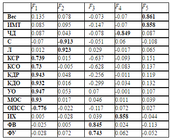
2. («» )

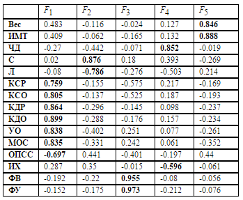
3. ( )

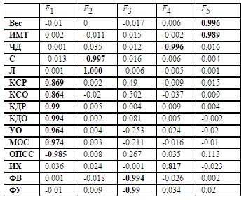
, «» . : 0, 1. , , , . , , . , .

, ( 4 ).

4 . ,

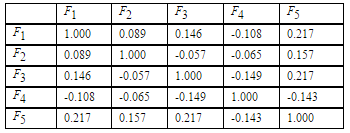
, . [ 1 3, 14]:

1. , , . , , . , , . , , . , . . , , , , .

2. (, ) . . , .

3. , .

4. , , .

5. , , . .

. , 3. 4 5 , . .

[13] . , , . , , . (- ) . , , . , , , .

. . . , : , . , .

. , , , «» .

1. . . . . . . ; . . . . — .: , 1980.

   
   

2. . . // . .: , 1994.

   
   

3. Hornik K., Stinchcombe M., White H. Multilayer Feedforward Networks are Universal Approximators. // Neural Networks, 1989, v.2, N.5.

   
   

4. Cybenko G. Approximation by Superpositions of a Sigmoidal Function. // Mathematics of Control, Signals and Systems, 1989, v.2.

   
   

5. Funahashi K. On the Approximate Realization of Continuous Mappings by Neural Networks. // Neural Networks. 1989, v .2, N .3, 4.

   
   

6. .. . // / . . . – , 1998. – .1, №1. – . 11-24.

   
   

7. C . : . . . . . , . . . 2- ., . — .: , 2008, 1103 .

   
   

8. . . .: , 2002, 344 .

   
   

9. Gorban A., Kegl B., Wunsch D., Zinovyev A., Principal Manifolds for Data Visualisation and Dimension Reduction // Springer, Berlin – Heidelberg – New York, 2007.

   
   

10. Kruger U., Antory D., Hahn J., Irwin GW, McCullough G. Introduction of a nonlinearity measure for principal component models. // Computers & Chemical Engineering, 29 (11-12), 2355–2362 (2005)

    
    

11. Jain AK, Mao J., Mohiuddin KM Artificial Neural Networks: A Tutorial. Computer, March, 1996, pp. 31-44.

    
    

12. .., .. . // . 2015. № 2. . 75-84.

    
    

13. Goltyapin V.V., Shoovin V.A. Oblique factorial model of first stage arterial hypertension. // Bulletin of Omsk University. 2010. No. 4. c . 120-128.

    
    

14. Chovin V.A. Confirmatory factor model of arterial hypertension. // Computer research and modeling. 2012. V. 4. No. 4. c . 885-894.