"Spherical trader in a vacuum": instructions for use

If you analyze

forums on markets (including Forex), we can distinguish two fairly stable opinions, let's call them pessimistic and optimistic:

Pessimists say: the market is random "because I built a random process chart and my friend (professional trader) could not distinguish it from the EURUSD chart", which means it is impossible to have a stable income on the market (Forex)!
')
Optimists object to them: if the market were random, the quotes would not have walked around 1, but went to infinity. So the market is not accidental and you can earn on it. I saw a really stable earning strategy with a large profit factor (more than that)!

Let's try to remain realistic and benefit from both opinions: suppose that the market is random, and based on this assumption, we construct a methodology for checking the profitability of the trading system for non-randomness .

The techniques considered in the article are universal for any markets, be it a fund, forex, or any other!

Formulation of the problem

Thanks to the well-known joke about a spherical horse in vacuum, a wonderful allegory was born, meaning an ideal, but completely inapplicable in practice model.

However, with the correct formulation of the problem, it is possible to extract quite tangible practical benefits by applying a "spherical model in vacuum." For example, through the denial of "sphericity" of the real object of study.

Suppose we have a trading system used in a certain market. Also suppose that the market is not accidental and the system uses something that is not a random number generator disguised as indicators for making trading decisions. To assess the stability of income, we use the profit factor: $PF = {P \ over L}$ where

- the amount of income, and

- amount of loss (positive number).

What should be the profit factor so that you can talk about the stability of this system? Obviously, the higher the profit factor, the more reasons to trust the system. But the lower limit is estimated by different experts in different ways. The most popular options are:> 2 (so-so),> 5 (good system),> 10 (great system). There is also such a variation: $PF_m = {P-p_m \ over L}$ where

- The maximum value of the income on the transaction, this value is called a reliable profit factor. It is believed that the minimum acceptable value for a reliable profit factor of 1.6.

What always confused me in the profit factor was the fact that the market dynamics and the intensity of trade are not taken into account. Therefore, I propose a different approach to assessing the significance of the profit factor, rather than a comparison with some a priori given value: the profit factor should be as high as possible, but not lower than the profit factor of a random system in a random market with similar trading intensity and volatility accordingly (in fact, not lower than that of the “spherical trader” in the “ideal gas” or in the “vacuum”).

It remains only to build an ideal model for comparison.

"Spherical trader ..."

Suppose we are considering some random trading system (“spherical trader”). Since the model is random, trading events occur at random points in time, regardless of the decisions made earlier. The direction of transactions is also random (with a probability of 0.5 sale or purchase). The volume of transactions is assumed constant, and without loss of generality, we estimate the profit and loss in points.

Let the average duration of the transaction is

, and the average time between closing two subsequent transactions

(we will not impose any restrictions on the number of simultaneously open transactions).

Also assume that we will deal with Poisson flows of events:

Transaction duration

will be a random variable with an exponential distribution:

$f (t) = \ lambda_te ^ {- \ lambda_tt} \ \ \ (1.1)$

Where

.

Amount of deals

committed over a period of time

will be described by the Poisson distribution:

$P_T (k) = {{\ left (\ lambda_ \ tau T \ right)} ^ k \ over k!} E ^ {- \ lambda_ \ tau T} \ \ \ (1.2)$

Where

"... in a vacuum"

Now consider the ideal habitat of the “spherical trader” - “vacuum”, that is, a completely random market.

Suppose that the market is described by the normal distribution of changes in the values of quotes

over a period of time

$f (\ Delta) = {1 \ over \ sigma_T \ sqrt {2 \ pi}} e ^ {\ Delta ^ 2 \ over {2 \ sigma_T ^ 2}} \ \ \ (2.1)$

Where

is determined as follows: let the quotes change for a unit time by a normally distributed random variable with variance

then, if we consider the time intervals

by changing the quotes will have a variance:

$\ sigma_T ^ 2 = \ sigma_1 ^ 2 T \\\ (2.2)$

This is a known correlation for the Brownian process.

Taking into account formulas (2.1) and (1.1), the result of the transaction, considered as a change in quotations over the period from the beginning to the end of the transaction, will be described as the integral of conditional probability

$f _ {\ sigma_1, \ lambda_t} (\ Delta) = \ int \ limits_ {0} ^ {\ infty} {\ lambda_t \ over {\ sigma_1 \ sqrt {2 \ pi t}}} e ^ {- {\ Delta ^ 2 \ over {2 \ sigma_1 ^ 2 t}}} e ^ {- \ lambda_tt} dt$

$f _ {\ sigma_1, \ lambda_t} (\ Delta) = {\ lambda_t \ over {\ sigma_1 \ sqrt {2 \ pi}}} \ int \ limits_ {0} ^ {\ infty} t ^ {- {1 \ over 2}} e ^ {- {\ Delta ^ 2 \ over {2 \ sigma_1 ^ 2 t}}} e ^ {- \ lambda_tt} dt \ \ \ (2.3)$

Solving this integral using Wolfram Mathematica gives the following result:

$f _ {\ sigma_1, \ lambda_t} (\ Delta) = {1 \ over \ sqrt {2}} {\ sqrt {\ lambda_t} \ over \ sigma_1} e ^ {- \ sqrt {2} {\ sqrt {\ lambda_t } \ over \ sigma_1} | \ Delta |}$

$f _ {\ sigma_1, \ lambda_t} (\ Delta) = {\ alpha \ over 2} e ^ {- \ alpha | \ Delta |} \ \ \ (2.4)$

Where $\ alpha = {\ sqrt {2 \ lambda_t} \ over \ sigma_1}$ .

The resulting pattern is the distribution of Laplace .

Thus, the income or loss on a single transaction of a random system in a random market is described by the Laplace distribution, and the absolute value of the result

The transaction has an exponential distribution:

$f_ \ alpha (R) = \ alpha e ^ {- \ alpha R} \ \ \ (2.5)$

Where $\ alpha = {\ sqrt {2 \ lambda_t} \ over \ sigma_1}$ .

It is known that the exponential distribution is a special case of the chi-square distribution (

). This means that total income and total losses can be described as sums of random variables with a chi-squared distribution , which means that they themselves are chi-squared quantities.

Let it be done

profitable trades with results

and

unprofitable with absolute losses

. Then total income

(normalized to

) and total losses

(also normalized to

) will be described by chi-square distributions with degrees of freedom

and

respectively:

$f \ left (P_ \ alpha \ right) = \ chi_ {k_p} ^ 2 \ left ({P_ \ alpha \ right) \ \ \ (2.6)$

$f \ left (L_ \ alpha \ right) = \ chi_ {k_l} ^ 2 \ left ({L_ \ alpha \ right) \ \ \ (2.7)$

Where $P_ \ alpha = {1 \ over {2 \ alpha}} \ sum \ limits_ {i = 1} ^ {k_p} R_i ^ +$ and $L_ \ alpha = {1 \ over {2 \ alpha}} \ sum \ limits_ {i = 1} ^ {k_l} R_i ^ -$ .

the ratio of these values will be as follows:

${P_ \ alpha \ over {L_ \ alpha}} = {{{1 \ over {2 \ alpha}} \ sum \ limits_ {i = 1} ^ {k_p} R_i ^ +} \ over {{1 \ over { 2 \ alpha}} \ sum \ limits_ {i = 1} ^ {k_l} R_i ^ -}} = {{\ sum \ limits_ {i = 1} ^ {k_p} R_i ^ +} \ over {\ sum \ limits_ {i = 1} ^ {k_l} R_i ^ -}} = {P \ over L} = PF \ \ \ (2.8)$

Where $P = \ sum \ limits_ {i = 1} ^ {k_p} R_i ^ +$ total income as well $L = \ sum \ limits_ {i = 1} ^ {k_l} R_i ^ -$ total losses. Their attitude

- profit factor.

Now consider the following value:

$PF_k = PF \ times {k_l \ over {k_p}} \ \ \ (2.9)$

This value can be interpreted as a “normalized profit factor”: the ratio of the average income to the average loss per transaction. Let's see what distribution this quantity has:

$PF_k = PF \ times {k_l \ over {k_p}} = {P \ over L} \ times {k_l \ over {k_p}} = {{P_ \ alpha} \ over {L_ \ alpha}} \ times {k_l \ over {k_p}} = {{{P_ \ alpha} \ over {2k_p}} \ over {{L_ \ alpha} \ over {2k_l}}} \ \ \ (2.10)$

The resulting quantity, the chi-squared ratio of the quantities normalized to the number of their degrees of freedom, has a Fisher distribution.

So we found the distribution of the magnitude, the statistics

for the profit factor "spherical trader in a vacuum" with a known amount of profitable

and unprofitable

deals.

Before proceeding to the generalization to the case of unknowns

and

Let us consider the behavior of the “spherical trader” in the “not entirely random” market (let's call this environment a joke “the ideal gas”).

"... in perfect gas"

Now consider a slightly more complicated situation: when the market is a generalized Brownian motion. That is, unlike the random, has a memory. In this case, formula (2.2) will take the following form:

$\ sigma_T ^ 2 = \ sigma_1 ^ 2 T ^ {2H} \ \ \ (3.1)$

Where

- Hurst index, a quantity characterizing the fractal properties of the time series and related to the fractal dimension of Hausdorff-Besicovitch

in the following way:

. Hurst's indicator can take values

.

With

the time series degenerates into a random, non-memory, corresponding to the case considered above. With

the series is constantly striving to change the direction of the existing trend, and therefore has a memory, such a series is called antipersistent, chaotic. With

the series also has a memory, but seeks to preserve the existing trend, such a series is called persistent, deterministic. The stronger the Hurst index is different from 0.5, the more clearly the chaotic or deterministic properties are expressed in the series.

Different markets are characterized by different values of the Hurst index, in addition, they may change from time to time. Hurst index can be calculated by the values of the time series. So, when evaluating the profit factor, you can take into account the value

calculated by a number of quotes in the same period when transactions of the analyzed strategy were made. There are several standard procedures for estimating the Hurst index, for example RS-statistics or wavelet-based methods.

Suppose that a random trading strategy works on the market with the Hurst index H, then, taking into account (3.1) , the formula (2.3) takes the form:

$f _ {\ sigma_1, \ lambda_t, H} (\ Delta) = {\ lambda_t \ over {\ sigma_1 \ sqrt {2 \ pi}}} \ int \ limits_ {0} ^ {\ infty} t ^ {- H} e ^ {- {\ Delta ^ 2 \ over {2 \ sigma_1 ^ 2 t ^ {2H}}}} e ^ {- \ lambda_tt} dt \ \ \ (3.2)$

Obviously, when

This expression is equivalent to (2.3) .

Unfortunately, expression (3.2) is not integrated analytically. Therefore, to find the distribution of the absolute values of the difference in quotations between the moments of the beginning and end of the transaction (absolute transactions) for random trading in the market with the Hurst index

we use numerical simulation.

I conducted simulations using Python.

The simulation is as follows.

1) Set the simulation parameters:

- the volume of the experimental sample;

- the number of ranges to build a histogram

2) Generate a sample distE of an exponentially distributed random variable and a sample distN of a normally distributed variable of volume N each.

3) Given the relation (3.1) , we create a test sample distT, each value of which is calculated from the corresponding distN and distE values:

4) For the distribution obtained, a histogram of M ranges is constructed (the number of hits in the ranges). From the obtained histogram, K first ranges are selected, the number of hits in which is different from zero. Also rationing is performed on the number of hits in the first range.

5) Based on the obtained histogram, the type of distribution is approximated.

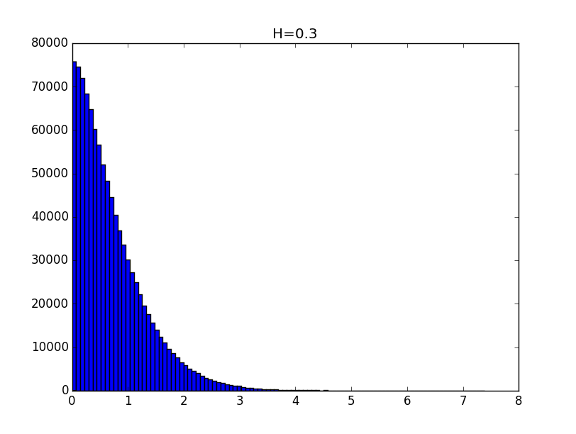
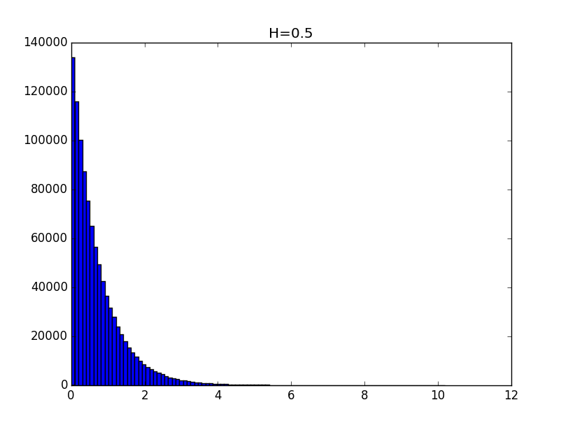
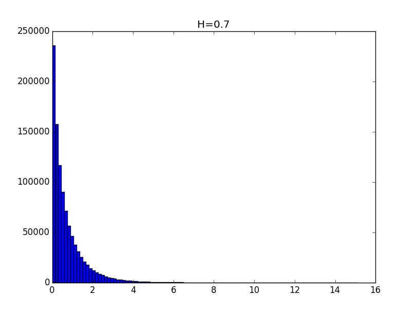
import matplotlib.pyplot as plt import numpy as np from scipy import stats def testH(N, M, H, p): distE = np.random.exponential(1, N) distN = np.random.normal(0, 1, N) distT = abs(distN * distE**H) if p == 1: plt.figure(1) plt.hist(distT, M) plt.title('H='+str(H)) [y, x] = np.histogram(distT, M) K = 0; for i in range(M): if y[i] > 0: K = i else: break y = y * 1.0 / y[0] x = x[1:K] y = y[1:K] return getCoeff(x, y, p, 'H='+str(H))

Examples of histograms of the obtained distributions for the values of the Hurst index 0.1, 0.3, 0.5, 0.7 and 0.9 are given below.

The general view of the histograms suggests that the obtained distributions, up to a constant, can be described by a function of the form:

$f _ {\ sigma_1, \ lambda_t, H} (\ Delta) = Ce ^ {- \ Delta ^ {K _ {\ sigma_1, \ lambda_t, H}}} \ \ \ (3.3)$

To search for the distribution parameter, we use the following algorithm:

1) Let us be given

- centroids of histogram ranges and

- the number of hits in the ranges normalized to the number hit in the first range.

2) Then, ignoring the first range, perform the conversion:

and

3) Using the method of least squares, we find the parameters of linear regression

and

such that

4) Based on received

accept:

.

Parameter

compensates for the error of normalization.

The listing of the procedure for calculating the coefficients is given below:

 def getCoeff(x, y, p, S): X = np.log(x) Y = np.log(-np.log(y)) n = len(X) k = (sum(X) * sum(Y) - n * sum(X * Y)) / (sum(X) ** 2 - n * sum(X ** 2)) b = (sum(Y) - k * sum(X)) / n if p == 1: plt.figure(2) plt.plot(np.exp(X), np.exp(-np.exp(Y)), 'b', np.exp(X), np.exp(-np.exp(k * X + b)), 'r') plt.title(S) plt.show() return k

The following are examples for envelopes of histograms for the Hurst values of 0.1, 0.3, 0.5, 0.7 and 0.9 (blue line) and their models (red line):

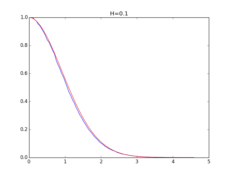
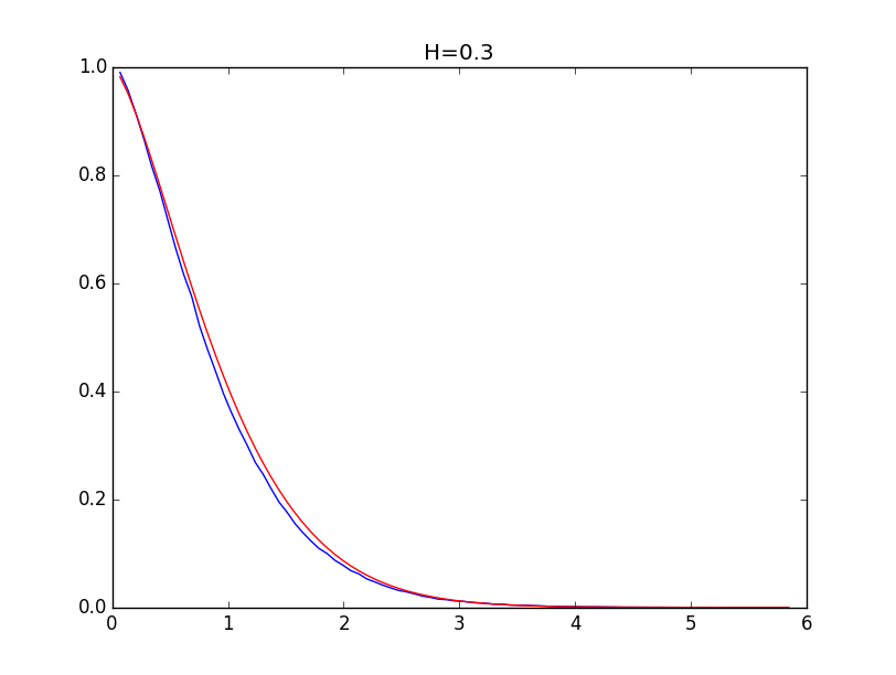
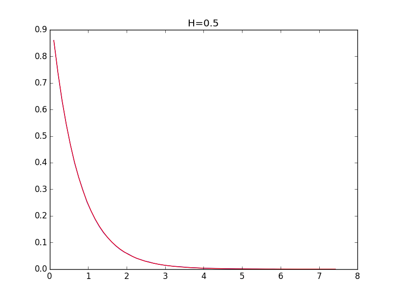
With the values of the Hurst index above 0.5, the simulation accuracy is higher.

Now we find the dependence

from

. To do this, we simulate a series of values

for various

and try to establish a functional dependency.

I used to simulate the values

from 0.01 to 0.99 in increments of 0.01. In addition, for each value

values

calculated 20 times and averaged:

 if __name__ == "__main__": N = 1000000; M = 100; Z = np.zeros((99, 2)) for i in range(99): Z[i, 0] = (i + 1) * 0.01 for j in range(20): W = float('nan') while np.isnan(W): W = testH(N, M, (i + 1) * 0.01, 0) Z[i, 1] += W Z[i, 1] *= 0.05 print Z[i, :] X = Z[:, 0].T Y = Z[:, 1].T plt.figure(1) plt.plot(X, Y) plt.show()

The resulting dependence is as follows:

The graph looks like a distorted sigmoid, so we will look for the pattern as a sigmoid:

$K (H) = d - {c \ over b + e ^ {a_3 H ^ 3 + a_2 H ^ 2 + a_1 H + a_0}} \ \ \ (3.4)$

A numerical minimization procedure using the least squares method gives the following results:

The total quadratic error is about 0.005.

Below are graphs of experimental dependence

(blue line) and model line according to formula (3.4) (red line):

It should be noted that the obtained pattern is valid only for the case when

and

. Therefore, in the future, we will assume that these conditions are fulfilled (we will ensure their fulfillment) and omit the corresponding indices.

Now, considering (3.3) and (3.4) for the estimated value

we know the distribution of the absolute value of transactions. Using the distribution property of the transformation of a random variable , we make the replacement of the variable in (3.4) :

Then:

$f_ {H} (\ Delta) = Ce ^ {- \ Delta ^ {K (H)}} >>> f '_ {H} (\ delta) = {C \ over K} \ delta ^ {{1 \ over {K (H)}} - 1} e ^ {- \ delta} \ \ \ (3.6)$

This is a probability density function of a quantity having a gamma distribution with a number of degrees of freedom.

and a single scale parameter. Given this, formula (3.6) . Must be rewritten as:

$f '_ {H} (\ delta) = {1 \ over {\ Gamma \ left ({1 \ over {K (H)}} \ right)}} \ delta ^ {{1 \ over {K (H) }} - 1} e ^ {- \ delta} \ \ (3.7)$

Let's summarize:

Having information about the Hearst Market Indicator

calculated for the same period of history on which we test the system, we can find the value

using formula (3.4) . We can also find the average trade intensity

and parameter

for transaction results. In order for the formulas proposed above to be valid, it is necessary to give the values

and

to unit. To do this, perform the normalization:

where

- result

transactions (regardless of the sign of the result). This transformation follows from (3.1) .

According to (3.7) , the values

will have gamma distributions with parameters

. Therefore, the values

will have a chi-square distribution c

degrees of freedom.

Let it be done

profitable transactions with income values

and

with loss values

(positive values). Then, taking into account

and (3.7) values

$P_H = 2 \ sum \ limits_ {i = 1} ^ {k_P} {(R_i ^ +)} ^ {K (H)}$

and

$L_H = 2 \ sum \ limits_ {i = 1} ^ {k_L} {(R_i ^ -)} ^ {K (H)}$

will have a chi-square distribution with quantities of degrees of freedom

and

respectively.

Therefore, the value:

$PF_H = {P_H \ over {L_H}} \ times {k_L \ over {k_P}} = {{\ sum \ limits_ {i = 1} ^ {k_P} {(R_i ^ +)} ^ {K (H)} } \ over {\ sum \ limits_ {i = 1} ^ {k_L} {(R_i ^ -)} ^ {K (H)}}} \ times {k_L \ over {k_P}} \ \ \ (3.8)$

will have a Fisher distribution c

degrees of freedom (the number of degrees of freedom, in general, will be non-integer, thus the fractal properties of the market are manifested).

Let's call the value

generalized normalized profit factor. With

the generalized profit factor degenerates into the normalized normal profit factor (2.9) .

Final summary

So, we investigated the “spherical trader” in a random market and found the distribution of the normalized profit factor. Then we summarized the results for the case of a market with an arbitrary fractal dimension, represented by a measurable quantity - the Hurst index.

Now we have a value that we call the generalized normalized profit factor, which is calculated using information on the results of transactions (by the way, let's not forget to correct them taking into account the spread: take it away from losses and add to income). For greater universality of the methodology, the volume of transactions is considered constant, or we measure everything in points. Do not forget also to carry out the normalization of the average duration of the transaction and the standard deviation of the distribution of the results of transactions:

where

- result

deal.

All the results obtained so far are tied to a known number of profitable and unprofitable transactions, which is a random variable with a binomial distribution for a known total number of transactions, which, in turn, is also a random variable distributed across Poisson .

We introduce a new designation. Let the generalized normalized profit factor (3.8) for a given amount of profitable

and the amount of unprofitable

transactions (with a known indicator of Hirst

) is denoted by

and has a Fisher distribution with degrees of freedom

.

Then, taking into account the binomial distribution of the number of profitable and unprofitable transactions, as well as the equal probability of receiving income or loss on each transaction, we introduce the value

- generalized normalized profit factor, taking into account only the total number of transactions. This value will have the following distribution:

$F_N (PF_ {H, N}) = \ left ({1 \ over 2} \ right) ^ N \ sum \ limits_ {k = 0} ^ {N} {\ left [{N! \ Over {k! ( Nk)!}} F_ {2kK (H), 2 (Nk) K (H)} (PF_ {H, N}) \ right]} \ \ \ (4.1)$

Where

- Fisher distribution density with degrees of freedom

and

and value

described by formula (3.4) , where

- Hurst figure.

In practice, with sufficiently large

expression (4.1) can be approximated by an incomplete sum:

$F_N (PF_ {H, N}) = {\ sum \ limits_ {k = a} ^ {b} {\ left [{N! \ Over {k! (Nk)!}} F_ {2kK (H), 2 (Nk) K (H)} (PF_ {H, N}) \ right]} \ over {\ sum \ limits_ {k = a} ^ {b} {N! \ Over {k! (Nk)!}} }} \ \ \ (4.1 *)$

Where

and

(

) limit a subset of the possible values of the number of profitable transactions.

Now we will consider the generalized normalized profit factor without reference to any number of transactions, but only taking into account the average trade intensity

and the testing period of the strategy

. Given that the total number of transactions is distributed by Poisson ,

will have the following distribution:

$PF _ {\ lambda_ \ tau, T, H} = \ sum \ limits_ {k = 0} ^ \ infty {{\ left (\ lambda_ \ tau T \ right) ^ k \ over {k!}} F_k (PF_ { H, N})} \ \ \ (4.2)$

Or, for the considered number of transactions in the range

$PF _ {\ lambda_ \ tau, T, H} = {\ sum \ limits_ {k = a} ^ b {{left (\ lambda_ \ tau T \ right) ^ k \ over {k!}} F_k (PF_ { H, N})} \ over {\ sum \ limits _ {k = a} ^ b {\ left (\ lambda_ \ tau T \ right) ^ k \ over {k!}}}} \ \ \ (4.2 * )$

The obtained distribution can be used to test the significance of the generalized normalized profit factor calculated by (3.8) for a trading system with a known average transaction duration and trading intensity for a certain amount of time in the market with known volatility and Hurst index. The method of application of the test is absolutely similar to that for the Fisher test. To carry it out, it suffices to replace in (4.1) (or (4.1 *) ) the density function with the Fisher distribution function and substitute the value of the calculated generalized profit factor as an argument. The resulting probability value must be compared with the value

where

- required level of significance. If this level is exceeded for the calculated statistics, one can reject the hypothesis about the randomness of the trading system (about the “sphericity of the trader in a vacuum”).

Conclusion

The proposed approach based on the construction of a generalized normalized profit factor, taking into account the volatility and fractal properties of the market, as well as the intensity of trade and the average duration of transactions, allows us to construct a statistical test of the significance of the results achieved in terms of the likelihood of similar results being obtained randomly. Using the test, it is possible with a given level of significance to talk about the fulfillment of the necessary condition for ascertaining the reliability of the system. But the results will not be a sufficient condition ...

Unfortunately, I do not know the test, the results of which will be sufficient for the unequivocal adoption of a strategy as unconditionally reliable.

Source: https://habr.com/ru/post/312096/

All Articles

"Spherical trader in a vacuum": instructions for use

Formulation of the problem

"Spherical trader ..."

"... in a vacuum"

"... in perfect gas"

Final summary

Conclusion

More articles: