Code Optimization: Memory
Most programmers represent the computing system as a processor that executes instructions, and a memory that stores instructions and data for the processor. In this simple model, the memory is represented by a linear array of bytes and the processor can access any place in memory for a constant time. Although it is an effective model for most situations, it does not reflect how modern systems actually work.
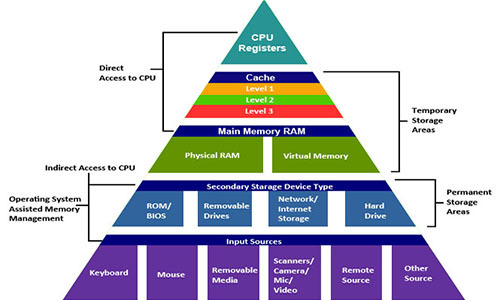
In fact, the memory system forms a hierarchy of storage devices with different capacities, cost, and access time. Processor registers store the most frequently used data. Small fast caches, located close to the processor, serve as buffer zones that store a small amount of data located in relatively slow RAM. RAM serves as a buffer for slow local disks. And local disks serve as a buffer for data from remote machines connected by a network.
The memory hierarchy works because well-written programs tend to access storage at a particular level more often than storage at a lower level. So storage at a lower level may be slower, larger and cheaper. As a result, we get a large amount of memory, which has the cost of storage at the very bottom of the hierarchy, but delivers data to the program at a speed of fast storage at the very top of the hierarchy.
As a programmer, you need to understand the memory hierarchy, because it greatly affects the performance of your programs. If you understand how the system moves data up and down the hierarchy, you can write programs that place their data higher in the hierarchy, so that the processor can access it faster.
')
In this article, we explore how storage devices are organized into a hierarchy. We especially focus on the cache memory, which serves as a buffer zone between the processor and the operational memory. It has the greatest impact on program performance. We will introduce the important concept of locality , learn how to analyze programs for locality, and also study techniques that will help increase the locality of your programs.
I was inspired to write this article by the sixth chapter from Computer Systems: A Programmer's Perspective . In another article in this series, “Code Optimization: The Processor,” we are also fighting for processor clock speeds.
Consider two functions that summarize the elements of a matrix. They are almost the same, only the first function bypasses the elements of the matrix line by line, and the second - in columns.
Both functions perform the same number of processor instructions. But on a machine with a Core i7 Haswell, the first function is performed 25 times faster for large matrices. This example well demonstrates that memory matters too . If you evaluate the effectiveness of programs only in terms of the number of instructions to be executed, you can write very slow programs.
Data has an important property that we call locality . When we work on the data, it is desirable that they are in the memory next. Traversing the matrix in columns has poor locality, because the matrix is stored in memory line by line. We'll talk about locality below.
The modern memory system forms a hierarchy from fast types of memory of small size to slow types of memory of large size. We say that a particular hierarchy level caches or is a cache for data located at a lower level. This means that it contains copies of data from a lower level. When the processor wants to get some data, it first searches for it at the fastest high levels. And goes down to the lower, if you can not find.
At the top of the hierarchy are the processor registers. Access to them takes 0 cycles, but there are only a few of them. Next comes a few kilobytes of first-level cache, access to which takes about 4 clock cycles. Then comes a couple of hundred kilobytes of a slower second-level cache. Then a few megabytes of third-level cache. It is much slower, but still faster than RAM. Next is a relatively slow RAM.
RAM can be considered as a cache for a local disk. Disks are workhorses among storage devices. They are big, slow and cheap. The computer loads files from disk into RAM when it is going to work on them. The gap in access time between the RAM and the disk is enormous. The disk is tens of thousands of times slower than RAM, and millions of times slower than the first level cache. It is more profitable to turn several thousand times to RAM than once to a disk. This knowledge is supported by data structures such as B-trees , which try to place more information in the RAM, trying to avoid accessing the disk at any cost.
The local disk itself can be considered as a cache for data located on remote servers. When you visit a website, your browser saves images from a web page to disk, so that when you visit them again you don’t need to download them. There are lower memory hierarchies. Large data centers, such as Google, store large amounts of data on tape media that is stored somewhere in warehouses and, when needed, must be attached manually or by a robot.
The modern system has approximately the following characteristics:
Fast memory is very expensive, and slow is very cheap. This is the great idea of system architects to combine large sizes of slow and cheap memory with small sizes fast and expensive. Thus, the system can operate at fast memory speeds and have a slow cost. Let's see how this works out.
Suppose your computer has 8 GB of RAM and a 1000 GB disk. But think that you do not work with all the data on the disk at one time. You load the operating system, open a web browser, text editor, a couple of other applications, and work with them for several hours. All these applications are placed in RAM, so your system does not need to access the disk. Then, of course, you close one application and open another, which you have to load from disk into RAM. But it takes a couple of seconds, after which you work with this application for several hours without accessing the disk. You do not particularly notice the slow disk, because at one moment you are working only with a small amount of data that is cached in RAM. It makes no sense for you to spend huge amounts of money on installing 1024 GB of RAM into which you could load the contents of the entire disk. If you had done this, you would have hardly noticed any difference in the work, it would be “money down the drain.”
The same is true for small processor caches. Suppose you need to perform calculations on an array that contains 1000 elements of type int . Such an array occupies 4 KB and is completely placed in the cache of the first level with a size of 32 KB. The system understands that you started working with a certain piece of RAM. It copies this piece into the cache, and the processor quickly performs actions on this array, enjoying the speed of the cache. Then the modified array from the cache is copied back into RAM. Increasing the speed of the RAM to the speed of the cache would not give a tangible increase in performance, but would increase the cost of the system hundreds and thousands of times. But all this is true only if the programs have good locality.
Locality is the main concept of this article. As a rule, programs with good locality run faster than programs with poor locality. Locality is of two types. When we refer to the same place in memory many times, it is temporary locality . When we access data, and then we access other data that are located in memory next to the original data, this is spatial locality .
Consider a program that summarizes the elements of an array:
In this program, the call to the variables sum and i occurs at each iteration of the loop. They have good temporal locality and will be located in fast processor registers. Elements of array A have a bad temporal locality, because we refer to each element only once. But then they have good spatial locality - by touching one element, we then touch the elements next to it. All data in this program have either good temporal locality or good spatial locality, so we say that the program generally has good locality.
When the processor reads data from memory, it copies it to its cache, while deleting other data from the cache. What kind of data he chooses to delete the topic is difficult. But the result is that if you frequently access some data, they are more likely to remain in the cache. This is a benefit from temporal locality. It is better for the program to work with fewer variables and access them more often.
Data movement between levels of hierarchy is performed by blocks of a certain size. For example, the Core i7 Haswell processor moves data between its caches in blocks of 64 bytes. Consider a specific example. We run the program on a machine with the above processor. We have an array of v containing 8-byte elements of type long . And we sequentially go around the elements of this array in a loop. When we read v [0] , it is not in the cache, the processor reads it from RAM to the cache with a block of 64 bytes in size. That is, elements v [0] - v [7] are sent to the cache. Next we go around the elements v [1] , v [2] , ..., v [7] . All of them will be in the cache and we will get access to them quickly. Then we read the element v [8] , which is not in the cache. The processor copies the elements v [8] - v [15] into the cache. We quickly go around these elements, but do not find the element v in the cache [16] . And so on.
Therefore, if you read some bytes from memory, and then read the bytes next to them, they will most likely be in the cache. This is a benefit of spatial locality. It is necessary to strive at each stage of the calculation to work with the data that are located in the memory nearby.
It is advisable to bypass the array sequentially by reading its elements one by one. If you need to bypass the elements of the matrix, it is better to bypass the matrix line by line, rather than in columns. This gives a good spatial locality. Now you can understand why the matrixsum2 function was slower than the matrixsum1 function. The two-dimensional array is located in memory line by line: first the first line is located, immediately after it comes the second one and so on. The first function read the elements of the matrix line by line and moved sequentially from memory, as if bypassing one large one-dimensional array. This function basically read the data from the cache. The second function went from line to line, reading one element at a time. She seemed to leap from memory from left to right, then return to the beginning and again start jumping from left to right. At the end of each iteration, she clogged the cache with the last lines, so she did not find the first lines at the beginning of the next iteration. This function basically read data from RAM.
As programmers, you should try to write code that is cache-friendly . As a rule, the main volume of calculations is performed only in a few places of the program. Usually these are several key functions and loops. If there are nested loops, then attention should be focused on the innermost of the loops, because the code is executed there most often. These places of the program also need to be optimized, trying to improve their locality.
Matrix calculations are very important in signal analysis and scientific computing applications. If programmers have the task to write the matrix multiplication function, then 99.9% of them will write it like this:
This code literally repeats the mathematical definition of matrix multiplication. We go around all the elements of the final matrix line by line, calculating each of them one by one. There is one inefficiency in the code; this is the expression B [k] [j] in the innermost loop. We go around matrix B by columns. It would seem that nothing can be done about it and will have to accept. But there is a way out. You can rewrite the same calculation differently:
Now the function looks very strange. But she does absolutely the same thing. Only we do not compute each element of the final matrix at a time; we sort of calculate the elements partly at each iteration. But the key feature of this code is that in the internal loop we go around both matrices line by line. On the machine with the Core i7 Haswell, the second function works 12 times faster for large matrices. You need to be a really wise programmer to organize the code in this way.
There is a technique called blocking . Suppose you need to perform a calculation on a large amount of data that does not all fit in the high-level cache. You break this data into smaller blocks, each of which is cached. Perform calculations on these blocks separately and then combine the result.
You can demonstrate this by example. Suppose you have a directed graph presented in the form of an adjacency matrix. This is such a square matrix of zeros and ones, so that if the element of the matrix with the index (i, j) is equal to one, then there is a face from the vertex of the graph i to the vertex j . You want to turn this directed graph into undirected. That is, if there is a face (i, j) , then the opposite face (j, i) should appear. Note that if the matrix is represented visually, then the elements (i, j) and (j, i) are symmetric with respect to the diagonal. This transformation is easy to implement in the code:
Blocking appears naturally. Imagine a large square matrix in front of you. Now excise this matrix with horizontal and vertical lines to split it into, say, 16 equal blocks (four rows and four columns). Select any two symmetric blocks. Please note that all elements in one block have their own symmetrical elements in another block. This suggests that the same operation can be performed on these blocks in turn. In this case, at each stage we will work only with two blocks. If the blocks are made small enough, they will fit in the high level cache. Express this idea in code:
It should be noted that blocking does not improve performance on systems with powerful processors that do a good prefetch. On systems that do not prefetch, blocking can greatly increase performance.
On a machine with a Core i7 Haswell processor, the second function does not run faster. On a machine with a simpler Pentium 2117U processor, the second function is performed 2 times faster . On machines that do not prefetch, performance would improve even more.
Everyone knows from the courses on algorithms that you need to choose good algorithms with the least complexity and avoid bad algorithms with high complexity. But these difficulties evaluate the execution of the algorithm on a theoretical machine created by our thought. On real machines, a theoretically bad algorithm can run faster than a theoretically good one. Remember that getting data from RAM takes 200 ticks, and 4 ticks from the first level cache is 50 times faster. If a good algorithm often touches memory, and a bad algorithm places its data in the cache, a good algorithm can run slower than a bad one. Also, a good algorithm can run worse on a processor than a bad one. For example, a good algorithm introduces data dependency and cannot load a processor pipeline. A bad algorithm is deprived of this problem and sends a new instruction to the pipeline on every clock cycle. In other words, the complexity of the algorithm is not all. How the algorithm will run on a specific machine with specific data matters.
Imagine that you need to implement a queue of integers, and new elements can be added to any position in the queue. You choose between two implementations: an array and a linked list.To add an element to the middle of the array, you need to move half the array to the right, which takes linear time. To add an element to the middle of the list, you need to go through the list to the middle, which also takes linear time. You think that since they have the same complexity, it is better to choose a list. Moreover, the list has one good property. The list can grow without limit, and the array will have to expand when it is full.
Suppose we have implemented a queue with a length of 1000 elements in both ways. And we need to insert an item in the middle of the queue. The elements of the list are randomly scattered in memory, so to get around 500 elements, we need 500 * 200 = 100'000 cycles. The array is located in memory sequentially, which allows us to enjoy the first-level cache speed. Using several optimizations, we can move the elements of the array, spending 1-4 clocks per element. We will move half of the array to a maximum of 500 * 4 = 2000 cycles. That is 50 times faster .
If in the previous example all the additions were to the top of the queue, the implementation with a linked list would be more efficient. If a fraction of the additions would be somewhere in the middle of the queue, implementing as an array could be the best choice. We would spend tacts on some operations and save tacts on others. And in the end, you could have won.
The memory system is organized as a hierarchy of storage devices with small and fast devices at the top of the hierarchy and large and slow devices at the bottom. Programs with good locality work with data from processor caches. Programs with poor locality work with data from relatively slow RAM.
Programmers who understand the nature of the memory hierarchy can structure their programs so that the data is located as high as possible in the hierarchy and the processor receives them faster.
In particular, the following techniques are recommended:
In fact, the memory system forms a hierarchy of storage devices with different capacities, cost, and access time. Processor registers store the most frequently used data. Small fast caches, located close to the processor, serve as buffer zones that store a small amount of data located in relatively slow RAM. RAM serves as a buffer for slow local disks. And local disks serve as a buffer for data from remote machines connected by a network.
The memory hierarchy works because well-written programs tend to access storage at a particular level more often than storage at a lower level. So storage at a lower level may be slower, larger and cheaper. As a result, we get a large amount of memory, which has the cost of storage at the very bottom of the hierarchy, but delivers data to the program at a speed of fast storage at the very top of the hierarchy.
As a programmer, you need to understand the memory hierarchy, because it greatly affects the performance of your programs. If you understand how the system moves data up and down the hierarchy, you can write programs that place their data higher in the hierarchy, so that the processor can access it faster.
')
In this article, we explore how storage devices are organized into a hierarchy. We especially focus on the cache memory, which serves as a buffer zone between the processor and the operational memory. It has the greatest impact on program performance. We will introduce the important concept of locality , learn how to analyze programs for locality, and also study techniques that will help increase the locality of your programs.
I was inspired to write this article by the sixth chapter from Computer Systems: A Programmer's Perspective . In another article in this series, “Code Optimization: The Processor,” we are also fighting for processor clock speeds.
Memory matters too
Consider two functions that summarize the elements of a matrix. They are almost the same, only the first function bypasses the elements of the matrix line by line, and the second - in columns.
int matrixsum1(int size, int M[][size]) { int sum = 0; for (int i = 0; i < size; i++) { for (int j = 0; j < size; j++) { sum += M[i][j]; // } } return sum; } int matrixsum2(int size, int M[][size]) { int sum = 0; for (int i = 0; i < size; i++) { for (int j = 0; j < size; j++) { sum += M[j][i]; // } } return sum; } Both functions perform the same number of processor instructions. But on a machine with a Core i7 Haswell, the first function is performed 25 times faster for large matrices. This example well demonstrates that memory matters too . If you evaluate the effectiveness of programs only in terms of the number of instructions to be executed, you can write very slow programs.
Data has an important property that we call locality . When we work on the data, it is desirable that they are in the memory next. Traversing the matrix in columns has poor locality, because the matrix is stored in memory line by line. We'll talk about locality below.
Memory hierarchy
The modern memory system forms a hierarchy from fast types of memory of small size to slow types of memory of large size. We say that a particular hierarchy level caches or is a cache for data located at a lower level. This means that it contains copies of data from a lower level. When the processor wants to get some data, it first searches for it at the fastest high levels. And goes down to the lower, if you can not find.
At the top of the hierarchy are the processor registers. Access to them takes 0 cycles, but there are only a few of them. Next comes a few kilobytes of first-level cache, access to which takes about 4 clock cycles. Then comes a couple of hundred kilobytes of a slower second-level cache. Then a few megabytes of third-level cache. It is much slower, but still faster than RAM. Next is a relatively slow RAM.
RAM can be considered as a cache for a local disk. Disks are workhorses among storage devices. They are big, slow and cheap. The computer loads files from disk into RAM when it is going to work on them. The gap in access time between the RAM and the disk is enormous. The disk is tens of thousands of times slower than RAM, and millions of times slower than the first level cache. It is more profitable to turn several thousand times to RAM than once to a disk. This knowledge is supported by data structures such as B-trees , which try to place more information in the RAM, trying to avoid accessing the disk at any cost.
The local disk itself can be considered as a cache for data located on remote servers. When you visit a website, your browser saves images from a web page to disk, so that when you visit them again you don’t need to download them. There are lower memory hierarchies. Large data centers, such as Google, store large amounts of data on tape media that is stored somewhere in warehouses and, when needed, must be attached manually or by a robot.
The modern system has approximately the following characteristics:
| Cache type | Access time (cycles) | Cache size |
|---|---|---|
| Registers | 0 | dozens of pieces |
| L1 cache | four | 32 KB |
| L2 cache | ten | 256 KB |
| L3 cache | 50 | 8 MB |
| RAM | 200 | 8 GB |
| Disk buffer | 100'000 | 64 MB |
| Local disk | 10'000'000 | 1000 GB |
| Remote servers | 1'000'000'000 | ∞ |
Fast memory is very expensive, and slow is very cheap. This is the great idea of system architects to combine large sizes of slow and cheap memory with small sizes fast and expensive. Thus, the system can operate at fast memory speeds and have a slow cost. Let's see how this works out.
Suppose your computer has 8 GB of RAM and a 1000 GB disk. But think that you do not work with all the data on the disk at one time. You load the operating system, open a web browser, text editor, a couple of other applications, and work with them for several hours. All these applications are placed in RAM, so your system does not need to access the disk. Then, of course, you close one application and open another, which you have to load from disk into RAM. But it takes a couple of seconds, after which you work with this application for several hours without accessing the disk. You do not particularly notice the slow disk, because at one moment you are working only with a small amount of data that is cached in RAM. It makes no sense for you to spend huge amounts of money on installing 1024 GB of RAM into which you could load the contents of the entire disk. If you had done this, you would have hardly noticed any difference in the work, it would be “money down the drain.”
The same is true for small processor caches. Suppose you need to perform calculations on an array that contains 1000 elements of type int . Such an array occupies 4 KB and is completely placed in the cache of the first level with a size of 32 KB. The system understands that you started working with a certain piece of RAM. It copies this piece into the cache, and the processor quickly performs actions on this array, enjoying the speed of the cache. Then the modified array from the cache is copied back into RAM. Increasing the speed of the RAM to the speed of the cache would not give a tangible increase in performance, but would increase the cost of the system hundreds and thousands of times. But all this is true only if the programs have good locality.
Locality
Locality is the main concept of this article. As a rule, programs with good locality run faster than programs with poor locality. Locality is of two types. When we refer to the same place in memory many times, it is temporary locality . When we access data, and then we access other data that are located in memory next to the original data, this is spatial locality .
Consider a program that summarizes the elements of an array:
int sum(int size, int A[]) { int i, sum = 0; for (i = 0; i < size; i++) sum += A[i]; return sum; } In this program, the call to the variables sum and i occurs at each iteration of the loop. They have good temporal locality and will be located in fast processor registers. Elements of array A have a bad temporal locality, because we refer to each element only once. But then they have good spatial locality - by touching one element, we then touch the elements next to it. All data in this program have either good temporal locality or good spatial locality, so we say that the program generally has good locality.
When the processor reads data from memory, it copies it to its cache, while deleting other data from the cache. What kind of data he chooses to delete the topic is difficult. But the result is that if you frequently access some data, they are more likely to remain in the cache. This is a benefit from temporal locality. It is better for the program to work with fewer variables and access them more often.
Data movement between levels of hierarchy is performed by blocks of a certain size. For example, the Core i7 Haswell processor moves data between its caches in blocks of 64 bytes. Consider a specific example. We run the program on a machine with the above processor. We have an array of v containing 8-byte elements of type long . And we sequentially go around the elements of this array in a loop. When we read v [0] , it is not in the cache, the processor reads it from RAM to the cache with a block of 64 bytes in size. That is, elements v [0] - v [7] are sent to the cache. Next we go around the elements v [1] , v [2] , ..., v [7] . All of them will be in the cache and we will get access to them quickly. Then we read the element v [8] , which is not in the cache. The processor copies the elements v [8] - v [15] into the cache. We quickly go around these elements, but do not find the element v in the cache [16] . And so on.
Therefore, if you read some bytes from memory, and then read the bytes next to them, they will most likely be in the cache. This is a benefit of spatial locality. It is necessary to strive at each stage of the calculation to work with the data that are located in the memory nearby.
It is advisable to bypass the array sequentially by reading its elements one by one. If you need to bypass the elements of the matrix, it is better to bypass the matrix line by line, rather than in columns. This gives a good spatial locality. Now you can understand why the matrixsum2 function was slower than the matrixsum1 function. The two-dimensional array is located in memory line by line: first the first line is located, immediately after it comes the second one and so on. The first function read the elements of the matrix line by line and moved sequentially from memory, as if bypassing one large one-dimensional array. This function basically read the data from the cache. The second function went from line to line, reading one element at a time. She seemed to leap from memory from left to right, then return to the beginning and again start jumping from left to right. At the end of each iteration, she clogged the cache with the last lines, so she did not find the first lines at the beginning of the next iteration. This function basically read data from RAM.
Cache-friendly code
As programmers, you should try to write code that is cache-friendly . As a rule, the main volume of calculations is performed only in a few places of the program. Usually these are several key functions and loops. If there are nested loops, then attention should be focused on the innermost of the loops, because the code is executed there most often. These places of the program also need to be optimized, trying to improve their locality.
Matrix calculations are very important in signal analysis and scientific computing applications. If programmers have the task to write the matrix multiplication function, then 99.9% of them will write it like this:
void matrixmult1(int size, double A[][size], double B[][size], double C[][size]) { double sum; for (int i = 0; i < size; i++) for (int j = 0; j < size; j++) { sum = 0.0; for (int k = 0; k < size; k++) sum += A[i][k]*B[k][j]; C[i][j] = sum; } } This code literally repeats the mathematical definition of matrix multiplication. We go around all the elements of the final matrix line by line, calculating each of them one by one. There is one inefficiency in the code; this is the expression B [k] [j] in the innermost loop. We go around matrix B by columns. It would seem that nothing can be done about it and will have to accept. But there is a way out. You can rewrite the same calculation differently:
void matrixmult2(int size, double A[][size], double B[][size], double C[][size]) { double r; for (int i = 0; i < size; i++) for (int k = 0; k < size; k++) { r = A[i][k]; for (int j = 0; j < size; j++) C[i][j] += r*B[k][j]; } } Now the function looks very strange. But she does absolutely the same thing. Only we do not compute each element of the final matrix at a time; we sort of calculate the elements partly at each iteration. But the key feature of this code is that in the internal loop we go around both matrices line by line. On the machine with the Core i7 Haswell, the second function works 12 times faster for large matrices. You need to be a really wise programmer to organize the code in this way.
Blocking
There is a technique called blocking . Suppose you need to perform a calculation on a large amount of data that does not all fit in the high-level cache. You break this data into smaller blocks, each of which is cached. Perform calculations on these blocks separately and then combine the result.
You can demonstrate this by example. Suppose you have a directed graph presented in the form of an adjacency matrix. This is such a square matrix of zeros and ones, so that if the element of the matrix with the index (i, j) is equal to one, then there is a face from the vertex of the graph i to the vertex j . You want to turn this directed graph into undirected. That is, if there is a face (i, j) , then the opposite face (j, i) should appear. Note that if the matrix is represented visually, then the elements (i, j) and (j, i) are symmetric with respect to the diagonal. This transformation is easy to implement in the code:
void convert1(int size, int G[][size]) { for (int i = 0; i < size; i++) for (int j = 0; j < size; j++) G[i][j] = G[i][j] | G[j][i]; } Blocking appears naturally. Imagine a large square matrix in front of you. Now excise this matrix with horizontal and vertical lines to split it into, say, 16 equal blocks (four rows and four columns). Select any two symmetric blocks. Please note that all elements in one block have their own symmetrical elements in another block. This suggests that the same operation can be performed on these blocks in turn. In this case, at each stage we will work only with two blocks. If the blocks are made small enough, they will fit in the high level cache. Express this idea in code:
void convert2(int size, int G[][size]) { int block_size = size / 12; // 12*12 // , for (int ii = 0; ii < size; ii += block_size) { for (int jj = 0; jj < size; jj += block_size) { int i_start = ii; // i [ii, ii + block_size) int i_end = ii + block_size; int j_start = jj; // j [jj, jj + block_size) int j_end = jj + block_size; // for (int i = i_start; i < i_end; i++) for (int j = j_start; j < j_end; j++) G[i][j] = G[i][j] | G[j][i]; } } } It should be noted that blocking does not improve performance on systems with powerful processors that do a good prefetch. On systems that do not prefetch, blocking can greatly increase performance.
On a machine with a Core i7 Haswell processor, the second function does not run faster. On a machine with a simpler Pentium 2117U processor, the second function is performed 2 times faster . On machines that do not prefetch, performance would improve even more.
What algorithms are faster
Everyone knows from the courses on algorithms that you need to choose good algorithms with the least complexity and avoid bad algorithms with high complexity. But these difficulties evaluate the execution of the algorithm on a theoretical machine created by our thought. On real machines, a theoretically bad algorithm can run faster than a theoretically good one. Remember that getting data from RAM takes 200 ticks, and 4 ticks from the first level cache is 50 times faster. If a good algorithm often touches memory, and a bad algorithm places its data in the cache, a good algorithm can run slower than a bad one. Also, a good algorithm can run worse on a processor than a bad one. For example, a good algorithm introduces data dependency and cannot load a processor pipeline. A bad algorithm is deprived of this problem and sends a new instruction to the pipeline on every clock cycle. In other words, the complexity of the algorithm is not all. How the algorithm will run on a specific machine with specific data matters.
Imagine that you need to implement a queue of integers, and new elements can be added to any position in the queue. You choose between two implementations: an array and a linked list.To add an element to the middle of the array, you need to move half the array to the right, which takes linear time. To add an element to the middle of the list, you need to go through the list to the middle, which also takes linear time. You think that since they have the same complexity, it is better to choose a list. Moreover, the list has one good property. The list can grow without limit, and the array will have to expand when it is full.
Suppose we have implemented a queue with a length of 1000 elements in both ways. And we need to insert an item in the middle of the queue. The elements of the list are randomly scattered in memory, so to get around 500 elements, we need 500 * 200 = 100'000 cycles. The array is located in memory sequentially, which allows us to enjoy the first-level cache speed. Using several optimizations, we can move the elements of the array, spending 1-4 clocks per element. We will move half of the array to a maximum of 500 * 4 = 2000 cycles. That is 50 times faster .
If in the previous example all the additions were to the top of the queue, the implementation with a linked list would be more efficient. If a fraction of the additions would be somewhere in the middle of the queue, implementing as an array could be the best choice. We would spend tacts on some operations and save tacts on others. And in the end, you could have won.
Conclusion
The memory system is organized as a hierarchy of storage devices with small and fast devices at the top of the hierarchy and large and slow devices at the bottom. Programs with good locality work with data from processor caches. Programs with poor locality work with data from relatively slow RAM.
Programmers who understand the nature of the memory hierarchy can structure their programs so that the data is located as high as possible in the hierarchy and the processor receives them faster.
In particular, the following techniques are recommended:
- Concentrate your attention on internal cycles. This is where the largest amount of computations and memory accesses occurs.
- , , , .
- , , .
Source: https://habr.com/ru/post/312078/
All Articles