Women and murder: is there a relationship here? [part 1 of 2]

UPD Added R code ( gist ) to reproduce all the results
A study recently published in the prestigious scientific journal Human Nature found that the prevalence of women is associated with higher crime. The conclusion strongly contradicts the everyday notion that where men are, there are crimes. However, he finds support in relatively young theories of marital market formation.
Despite the slenderness of the methods used in the study, it seems to me that an important variable was missed in it, perhaps the key variable. It would be great to check on the same data, but the authors do not publish them as an appendix to the article, and collecting them yourself is quite a lot of work. So far I have decided to go another way - to eliminate the problem variable from the study design.
I checked whether there is a similar pattern in Europe at the country level. Interested please under the cat.
Initially, my attention to the study was attracted by a blog post by demographer Boris Denisov . In the discussion with him was born the idea to check the pattern in Europe. Checked The results are interesting. And he began to think where to publish. Once again, I came to the conclusion that there is no better option for the habr. I understand that the topic is likely to interest the smaller part of the audience of the community. And yet I hope for a benevolent attitude and valuable comments - I really want to hear opinions "from the side." As for the categorization of the article - I think, on the Habré, the Academy (the Academy) would not interfere with the hub (or even the stream) ( wrote from this earlier in the commentary ).
In my defense, I can say that those who are not interested in demography will find in this post an R code that automatically downloads population data from two excellent databases - Eurostat and the Human Mortality Database and reproduces all charts, including maps. (Link to the code at the end of the article)
So, what confused me?
Schacht, R., Tharp, D., & Smith, K. (2016). Marriage markets and male mantra effort: violence and violence are elevated where men are rare. Human Nature, 1–12. https://doi.org/10.1007/s12110-016-9271-x
After examining the sex ratio in the adult population of the counties of the USA (more than 3 thousand administrative districts) and data on the commission of serious crimes, Ryan Schacht, Douglas Tharp and Ken Smith concluded that there is a clear correlation between the indicators - the more men, the fewer crimes ( Table 1).
Table 1. The results of a regression model describing the relationship between the homicide rate (per 100 thousand people) and the sex ratio at the age of 15-45 years. [N = 3082 counties, DF = 3077; −2loglikelihood = 12,372]
| Variable | Coefficient | Standard error | t | p-value |
|---|---|---|---|---|
| Intersection | 5.625 | 0,509 | 11.04 | <0.0001 |
| Sex ratio, 15-45 years | -0.033 | 0,003 | -9,50 | <0.0001 |
| Poverty rate (%) | 0.011 | 0,010 | -1.16 | 0.245 |
| White population ratio (%) | -0.041 | 0,003 | -12,86 | <0.0001 |
| North / South (0.1) | 0,940 | 0.122 | 7.72 | <0.0001 |
The conclusion strongly contradicts the notion that where men are, there are crimes. For decades this intuitive presentation has been rather groundless, or rather speculatively, dominated in sociological works. In contrast to these theoretical constructs, there are relatively recent theories that are based on modeling marriage markets that predict an inverse relationship. Recently revised sociological theories of marriage markets predict a negative effect from an excess of women and insufficient competition among men. The empirical research of Mine et al. Is consistent with this spiral of modern scientific literature. The logic is approximately the following: the abundance of women leads to a decrease in the efforts put by men to form pairs, which in turn leads to a disorderly life and a general increase in crime.
Despite the beauty of analyzing small areas (other things being equal, it is always more pleasant to analyze more fractional data), there are big doubts about the possible missing variable in the study - the division of American counties on the principle of centrality / peripherality (urban / rural).
The fact is that women are more active than men in internal migration. This is one of the laws of Ravenstein-Lee migration.
Original articles by Ernst-Georg Ravenstein.
- Ravenstein, EG (1885). The Laws of Migration. Journal of the Statistical Society of London, 2, 167. https://doi.org/10.2307/2979181
- Ravenstein, EG (1889). The Laws of Migration. Journal of the Royal Statistical Society, (2), 241. https://doi.org/10.2307/2979333
Article Everett Lee, staked out for Ravenstein right to be considered the father of migrationology.
- Lee, ES (1966). A theory of migration. Demography, 3 (1), 47–57. https://doi.org/10.2307/2060063
In Russian there is a good review article of my colleagues from the Institute of Demography of the HSE.
- Abylkalikov, S.I., & Vinnik, M.V. (2012). Economic theories of migration: labor and the labor market. Business. Society. Power, (12), 1–19. https://www.hse.ru/mag/27364712/2012--12/71249233.html
Due to this pattern in cities, the sex ratio is usually warped towards women. For illustration, here is a map of Russia from my master’s work (Fig. 1).
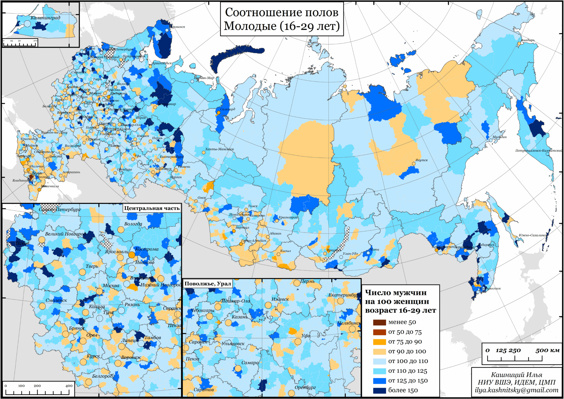
Figure 1. Sex ratio between the ages of 16-29 years in municipalities and cities of Russia according to the 2010 All-Russian Population Census. (clickable)
As we see, there are more women in cities (there are regional centers, where there are more men, but, as a rule, this is explained by military units — a separate topic). And this is despite the fact that there are always more boys born than girls, and at a young age there are more boys in general. But more on that later. So, thanks to internal migration, women are concentrated in cities.
And in the cities, crime is higher. There are a lot of reasons (mostly different sociological theories about isolation from the environment), but there is no need to prove this thesis.
So, in my opinion, in the study of Mine, Tharp and Smith, the key difference between the city and the periphery is probably missing. In cities, there is more crime because it is a city, and not because there are more women and less men. It is possible that the inclusion of the variable urban / rural in the explanatory model neutralizes the observed effect.
But in order to check whether this is so, one must have the same data that the researchers used. Probably do it sometime later. In the meantime, in the discussion we came to the conclusion that it would be interesting to check the revealed dependence on the data of European countries. The transition to the level of countries should largely solve the effects of migration.
Check on European data
So, the idea is to check the identified relationship on the data on population and crime of European countries. The transition to a higher level of data aggregation is intended to solve the issue of the classification of territories into central and peripheral.
Data
- population age structure - Human Mortality Database (we are interested in the Exposure-to-risk indicator);
- data on the number of murders in European countries - Eurostat (dataset of interest to us is called "crim_gen", it is easier to download here ).
Data from the two bases intersected in 28 countries (in fact, 26, just Scotland and Northern Ireland are present in the statistics separately). Not bad. There is data, then everything is simple. We calculate the ASR, adult sex ratio, the ratio of men to women aged 15-49 years (the authors of the Human Nature article use the age range 15-49 years; deviation from their methodology is dictated by the characteristics of Eurostat data) and HR, Homicide Rate, homicide rate per 100 Thousands of people of the local population.
Next is linear regression. I know that the authors use a more sophisticated statistical model, but for the beginning we will go in a simple way.
The fact is that the Poisson regression has a lot of meaning when there are many values in a large data array, close to zero or zero. For the analysis of American counties, this is indeed a significant difficulty. In our analysis of countries, it is quite possible to limit ourselves to a simple linear regression.
Who is interested in the question of the applicability of the Poisson regression for modeling processes with low probabilities (small coefficients), pay attention to the classic article.
- Welch, BL (1951). On the comparison of several mean values: an alternative approach. Biometrika, 330–336. Retrieved from http://www.jstor.org/stable/2332579
The method is widely applicable in epidemiology. I used Poisson regressions in my recent study of the influx of migrants to Moscow. There is just such a situation: when we consider migration flows separately for men / women, five-year age groups and 125 districts of the city, it often turns out that combinations of all signs give zero coefficients. Therefore, it is convenient to use Poisson regression. Who is interested in the article, here it is (free postprint here ):
- Kashnitsky, IS, & Gunko, MS (2016). Spatial variation of in-migration to Moscow: testing the effect of the housing market. Cities. https://doi.org/10.1016/j.cities.2016.05.025
But first look at the cards.
Here is the sex ratio between the ages of 15-49 years in European countries (hereinafter, Britain is given as a weighted average of the constituent parts - I was too lazy to look for spatial data and mess with it).

Figure 2 . Sex ratio between the ages of 15-49 in Europe
As you can see, the spread is quite large (just in case, there is data in Estonia and the UK, just the values are very close to 1). And this suggests the need for additional verification (but this is at the end of the article).
The prevalence of homicides in Europe varies greatly between East and West (Fig. 3). In the Baltic countries, the indicator is so much higher than in the rest of Europe (Fig. 3-A) that we have to exclude them (Fig. 3-B) from the regression analysis as outright emissions.

Figure 3 . Homicide rates, incidents per 100K population per year.
Finally, another variable included in the analysis by the authors of the original study is the proportion of the population below the poverty line. The map of European countries looks like this (Fig. 4).

Figure 4 . The proportion of the population below the poverty line.
Eliminating the Baltic countries, let's start, finally, the modeling.
Regression analysis
We simulate the homicide rate (hr) using data on the sex ratio at the age of 15-49 (asr), dummy variables for years and, in the second model, the proportion of people below the poverty line (pov). We get the following result (Table 2).
Table 2. Simulation results.
| Model 1 | Model 2 | ||
|---|---|---|---|
| (Intercept) | 98.94 (24.46) *** | 97.38 (04/20) *** | |
| asr | -0.80 (0.24) *** | -0.89 (0.20) *** | |
| year2001 | -0.73 (1.91) | -0.72 (1.57) | |
| year2002 | -0.75 (1.91) | -0.74 (1.57) | |
| year2003 | -2.26 (1.91) | -2.26 (1.57) | |
| year2004 | -1.69 (1.91) | -1.68 (1.57) | |
| year2005 | -3.47 (1.92) | -3.45 (1.57) * | |
| year2006 | -4.32 (1.92) * | -4.28 (1.57) ** | |
| year2007 | -3.51 (1.92) | -3.46 (1.57) * | |
| pov | 0.43 (0.04) *** | ||
| R 2 | 0.10 | 0.40 | |
| Adj. R 2 | 0.07 | 0.37 | |
| Num. obs. | 200 | 200 | |
| RMSE | 6.77 | 5.55 | |
| *** p <0.001, ** p <0.01, * p <0.05 | |||
It turns out, indeed, a lower sex ratio correlates with higher crime rates. And the poverty variable, while explaining a significant amount of variation in the data, does not neutralize the relationship between sex ratio and crime.

Figure 5. Correlation between the level of crime (murder) and the sex ratio in adulthood.
However, let us note that the sex ratio is significantly lower in Eastern Europe (Fig. 2) than in Western. Here we are likely to encounter once again the manifestation of the influence of migration, but this time migration is international. Another of the laws of migration Ravenstein-Lee argues that in international migration, by contrast, men are more active. It is possible that the results of my small verification were distorted from international migration. Verify by eliminating the effect of international migration.
Analysis by age structure from mortality tables
In order to eliminate the impact of international migration, we will resort to calculating the sex ratio from mortality tables, which can also be downloaded from the Human Mortality Database.
Mortality tables are a basic tool for demographers to study mortality. They simulate the extinction of a hypothetical generation. Suppose we calculate the CU for country A in the year X. The baseline is the age-specific mortality rate in the year X. Next, we model the extinction of the conditional generation (usually taken as 100K, but this is not important), assuming that to die with the intensity characteristic of the inhabitants of country A at the appropriate age in the year X.
The beauty of the CU is that the estimates based on it (the best known is life expectancy) do not depend on the age structure of the population. Thus, it is possible to correctly compare the mortality of completely different populations, for example, very old Japan and very young Nigeria.
Of course, the CU can be calculated separately for men and women, yes, in general, for any population - there would be data.
We calculate the sex ratio in adulthood as the ratio of the number of men and women according to the mortality table multiplied by the initial sex ratio at birth.
Boys are always and everywhere born more than girls. This is an immutable law of nature. On average, 106 boys are born per 100 girls.
In fairness, we note that, as a rule, male mortality is higher than female mortality at all ages. Therefore, at a certain age, the sex ratio is equalized.
This is how the average sex ratio at birth looked in our countries in 1990–2010 (Fig. 6).

Figure 6 . Primary sex ratio in European countries (A) and standard deviation of the indicator (B), 1990-2010.
As you can see, deviations from 106 are minor. However, I still consider them in further calculations.
Thus, we have obtained the sex ratio in adulthood, as it would have been if only mortality had influenced the number of generations. That is, migration is excluded from consideration. This is how our indicator looks on the map (Fig. 7).

Figure 7 . Sex ratio in adulthood based on estimates from mortality tables.
Finally, we calculate models with a new sex ratio in adulthood. With a similar analysis, we obtain the following models.
Table 3. Simulation results, sex ratio based on total mortality rates.
| Model 1 | Model 2 | ||
|---|---|---|---|
| (Intercept) | 503.99 (78.42) *** | 466.81 (63.99) *** | |
| asr_lt | -4.68 (0.75) *** | -4.41 (0.61) *** | |
| year2001 | -0.76 (1.80) | -0.76 (1.46) | |
| year2002 | -0.80 (1.80) | -0.80 (1.46) | |
| year2003 | -2.32 (1.80) | -2.32 (1.46) | |
| year2004 | -1.78 (1.80) | -1.78 (1.46) | |
| year2005 | -3.65 (1.80) * | -3.65 (1.46) * | |
| year2006 | -4.65 (1.80) * | -4.65 (1.46) ** | |
| year2007 | -3.96 (1.80) * | -3.96 (1.46) ** | |
| pov | 0.40 (0.04) *** | ||
| R 2 | 0.21 | 0.48 | |
| Adj. R 2 | 0.18 | 0.45 | |
| Num. obs. | 200 | 200 | |
| RMSE | 6.35 | 5.17 | |
| *** p <0.001, ** p <0.01, * p <0.05 | |||
We see that the coefficients with a variable sex ratio remained negative and increased significantly (pay attention to the scale on the X axis, Fig. 8).

Figure 8. Correlation between the level of crime (homicide) and the sex ratio in adulthood, calculated from mortality tables.
Intermediate output
The result did not meet my expectations. Neither the transition to the level of countries (to eliminate the effect of internal migration), nor the use of the sex ratio in the mortality tables (to eliminate the effect of international migration) did not change the nature of the relationship between homicide rates and sex ratio in adulthood.
The resulting modeling result using gender ratios, calculated from mortality tables, may indicate the presence of an inverse causal relationship (as suggested in 7ft comments). That is, the logic is: where there are more crimes, there are fewer men as a result of these very crimes.
Also in the discussion the idea was born (thanks, Ghedeon and dom1n1k for the discussion) to distribute a nice chart for all HMD countries (Fig. 9)
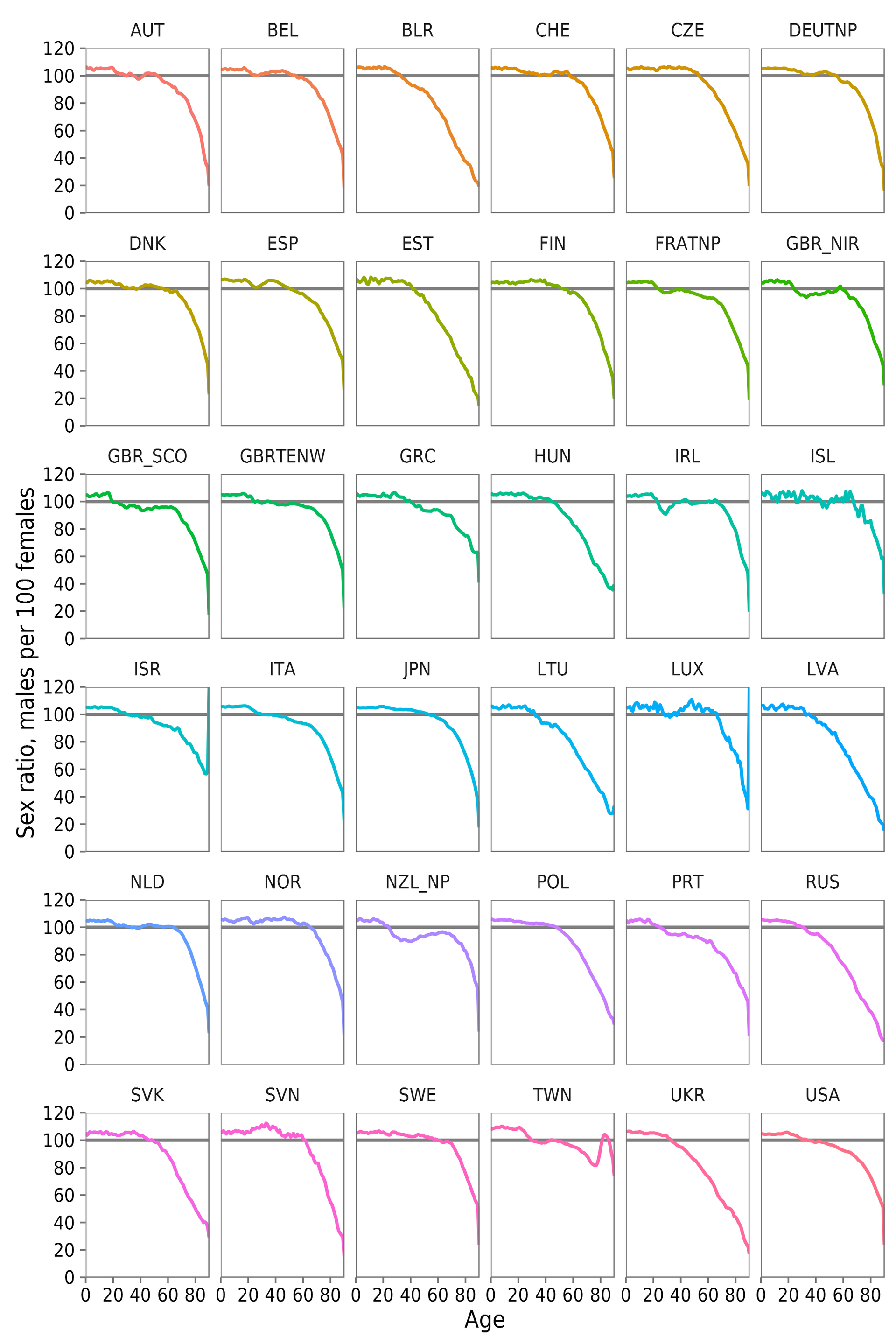
Figure 9. Sex ratios at all ages for all countries from the Human Mortality Database, 2012.
In the second part there will be a test of the hypothesis on the American data.
I would appreciate comments - probably missed something.
UPD 2016-10-12 18:45 Promised R code laid out on the gith link (gist) by reference
https://goo.gl/bhOmxp
(comments on the code are welcome)
UPD 2018 : all materials on github .
')
Source: https://habr.com/ru/post/311970/
All Articles