Chaos inside sudoku

Many of you are probably familiar with such a puzzle as sudoku. Perhaps even implemented a program for automatic solutions. On Habré, the topic of sudoku has already been discussed many times, and, as practice shows, almost any method of automatically finding an answer ultimately boils down to a targeted search. And this is quite natural, because even manual solutions adhere to the same principles. But what if you do otherwise?
In this article I will consider one very entertaining method proposed in 2012, based on a strictly mathematical approach. Software implementation is attached.

Stage 0. Task statement

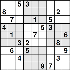
First of all, recall the description of the puzzle. The task of any Sudoku layout is to fill in a 9x9 field with numbers from 1 to 9 so that none of the rows, columns, or the selected 3x3 block contain the same numbers (blocks are marked with bold borders in the picture). The uniqueness of such a filling is usually also implied; this fact helps in solving problems of a high level of complexity. We (as well as brute force algorithms) do not require the assumption of the uniqueness of the solution. It is worth making a reservation: the described method allows you to find the first available solution. Enumeration of all solutions by this method is impossible (well, or at least impractical).

Stage 1. Task formalization

We describe mathematically what a correctly filled field is. We have a 9x9 grid, only one number from 1 to 9 can be located in each cell. It would be reasonable to enter 81 integer variables, but instead we will operate on boolean values. This will allow the use of a formal logical approach.

We introduce the set logical variables, giving them the following meaning: in a cage recorded number . Determining the correct field in sudoku dictates a number of constraints that we introduce on the set of our variables.

For simplicity, we first introduce the q-local predicate , true only if exactly one of its parameters is true. Here is its formal description:

With its help we will write down 4 types of the restrictions described by us earlier:

• in each cell there can be only one of 9 numbers:

• in each line each number occurs exactly 1 time:

• in each column, each number occurs exactly 1 time:

• The most unpleasant case to describe is that each of the 9 3x3 blocks contains each number exactly 1 time:

If we combine all the above formulas, getting rid of quantifiers, we get this:

This formula has a Conjunctive Normal Form (since the predicate also recorded in CNF), which is a very convenient way for software processing.

We have a general formula on our hands that describes all possible Sudoku fields. In practice, in the Sudoku field there are several tips. If in a cage worth the number then we know that . In addition, we can easily define many variables that must be false under these conditions. We substitute all these quantities and simplify each of the clauses. Further, we have the right to remove from the formula recurring clauses (if they appeared) and declare that the resulting function (still in CNF) fully determines our alignment, and each solution of the equation gives us a unique solution to the original problem. So, by and large, we reduced Sudoku to the classical problem of feasibility from mathematical logic. It is NP-complete, which to some extent explains the complexity of the original puzzle.

Stage 2. Some mathematical analysis

From this point on, it is possible to forget that we solve Sudoku, since the described method is suitable for any feasible task. And we will need several new notation to describe it.

Suppose there is a formula consisting of N logical variables and M disjunct. Introduce the matrix MxN size, such that:

• = 1 if the m-th disjunct contains ;
• = -1 if the m-th disjunction contains a negative ;
• = 0 if the m-th disjunction does not contain .

Next, we introduce the vector such that = {number of variables in disjunct number m}.
And in the end, everyone assign a real number . it is a continuous quantity which for is -1, and for equal to 1. In a sense .

Now you can figure out why all this is needed. We assign a function to each of the M disjunctions. defined as follows:

These functions are good because they are 0 (if one of the factors is zero) corresponding clause with corresponding values is true. Moreover, adding multipliers with ensures that each of the functions takes values ​​from the segment in the field of its definition. But the sum of their squares will be more interesting:

This sum is remarkable in that it vanishes exclusively on those vectors s that correspond to the solutions of the original equation on . And all these zeros are local minima of our function (due to the range of values).

Stage 3. The system of differential equations

The equation, despite the apparent simplicity of the record, in fact turns out to be very unpleasant. This is a large polynomial from a very large number of arguments. You can not even try to look for its minimum analytically.

Let's make some additions:

• imagine each as a function ;
• we introduce some more functions ;
• instead of our will consider

Since all strictly positive, then our equation does not lose its most important properties.
Wherein and We will find the following conditions:

∇ in this record is the gradient operator.

The first equation clearly hints at the conjugate gradient method for searching extremes.
With the second a little more cunning, I will leave it on the conscience of the authors. In short, it is necessary for the system to converge more quickly to a solution. I myself did not check whether this is true.

Equation for can be rewritten explicitly by differentiating V:

The initial conditions at point 0 are taken arbitrary. Well, the solution we end up with is the following formula:

Stage 4. Finally, the numerical solution

One of the easiest and most convenient ways to solve systems of ordinary differential equations is the Runge-Kutta method. We will use a variant of the method, bearing the names of Cash-Karp. Now I will talk about it briefly.

So, let us have the equation . x in the parameter list we omit, because in our equations the values ​​of the derivatives and Do not depend explicitly on t. It's easier for us.

We assume that the initial condition is given , and we need to find the value .
To find the answer, we will build a sequence and we will calculate the values .

and we know them, we consider them as the base of induction. Further, suppose we are at step n <N, we denote . Will seek based on the following formula:

in which the sequence is like:

Numbers , and are fixed constants on which the accuracy of the method depends strongly (in the canonical method there are also constants , but in our case they are simply not needed).
Together, the set of these coefficients is called the “Butcher table”:

For the Cash-Karp method, we have the following table:

Here we have two vectors b. If you use the first one, then at each step the calculation error is estimated as . And if we take the second vector b, then the error estimate will be . Considering a less accurate value , we can heuristically estimate the absolute error on the step as (the difference between the solutions of the 4th and 5th orders). And if the error does not suit us, we can replace the current step h with a different value and recalculate the current iteration. In particular, there are 2 options:

• too big mistake - we reduce the step, we start the iteration from the beginning;
• too small error - increment step, run the next iteration (thereby reducing the total computation time).

Stop the search process is possible when all calculated modulo will be slightly different from the unit (the difference in 0.1 is enough).

Conclusion

Well, definitely a bit of a fuss for such a simple task. Personally, I tried to sort out all this material solely out of curiosity, since I rarely meet such a wide use of mathematics in such unexpected places.

Does everything described above work in practice? The authors did not share the code, so I had to write my own.

He solves the problem, but for sudoku from the "most complex in the world" class it works very slowly, and the duration of the solution depends strongly on the initial data (that is, on the random number). I cannot answer with certainty whether this is a problem with the method or my implementation. There were no obvious bugs.

If you are really interested in this topic, I strongly advise you to read the original. I have not touched all the material considered by the authors of the method. And thank you for reading to the end!

References:

1. original publication on sudoku
2. general method for solving the feasibility problem
3. Cash-Karp method
4. my github implementation (java)