learnopengl. Lesson 1.4 - Hello Triangle

In the last lesson, we still mastered the opening of the window and the primitive user input. In this tutorial, we will analyze all the basics of displaying vertices on the screen and use all the features of OpenGL, like VAO, VBO, EBO, in order to display a pair of triangles.
Interested please under the cat.




In OpenGL, everything is in 3D space, but at the same time the screen and the window are a 2D matrix of pixels. Therefore, most of the work of OpenGL is the transformation of 3D coordinates into 2D space for drawing on the screen. The process of converting 3D coordinates to 2D coordinates is controlled by the OpenGL graphics pipeline. The graphics pipeline can be divided into 2 large parts: the first part converts the 3D coordinates to 2D coordinates, and the second part converts the 2D coordinates to color pixels. In this lesson we will discuss in detail the graphics pipeline and how we can use it as a plus to create beautiful pixels.

There is a difference between 2D coordinates and a pixel. A 2D coordinate is a very accurate representation of a point in 2D space, while a 2D pixel is an approximate location within your screen / window.

The graphics pipeline takes a set of 3D coordinates and converts them to color 2D pixels on the screen. This graphic container can be divided into several stages, where each stage requires the input of the result of the past. All these stages are extremely specialized and can easily be performed in parallel. Due to their parallel nature, most modern GPUs have thousands of small processors for fast processing of the graphics pipeline by running a large number of small programs at each stage of the pipeline. These small programs are called shaders .

Some of these shaders can be customized by the developer, which allows us to write our own shaders to replace the standard ones. This gives us much more opportunities to fine-tune specific areas of the pipeline, and it is because of the fact that they work on the GPU, which allows us to save processor time. Shaders are written in OpenGL Shading Language (GLSL) and we will delve more into it in the next lesson.

In the image below you can see an approximate representation of all stages of the graphics pipeline. The blue parts describe the stages for which we can specify our own shaders.



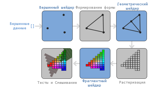
As you can see, the graphics pipeline contains a large number of sections, where each is engaged in its part of processing vertex data into a fully rendered pixel. We will describe each section of the conveyor a bit in a simplified way to give you a good idea of ​​how the conveyor works.

An array of 3D coordinates is transmitted to the input of the conveyor, from which triangles can be formed, called vertex data; vertex data is a collection of vertices. A vertex is a data set on top of a 3D coordinate. This data is represented using vertex attributes, which can contain any data, but for simplicity, we assume that the vertex consists of a 3D position and a color value.

Since OpenGL wants to know what to make of the collection of coordinates and color values ​​passed to it, OpenGL requires you to specify which shape you want to form from the data. Do we want to draw a set of points, a set of triangles, or just one long line? Such shapes are called primitives and are passed to OpenGL during the invocation of drawing commands. Some of the primitives are: GL_POINTS , GL_TRIANGLES and GL_LINE_STRIP .

The first stage of the pipeline is the vertex shader, which takes one vertex at the input. The main task of the vertex shader is to convert 3D coordinates to other 3D coordinates (more on this later) and the fact that we have the ability to change this shader allows us to perform some basic transformations on the values ​​of the vertex.

Assembly of primitives is a stage that takes as input all vertices (or one vertex if GL_POINTS primitive is selected ) from the vertex shader, which form the primitive and assembles the primitive from them; in our case it will be a triangle.

The result of the primitive assembly step is passed to the geometry shader. He, in turn, at the input accepts a set of vertices that form primitives and can generate other shapes by generating new vertices to form new (or other) primitives. For example, in our case, it will generate a second triangle in addition to this shape.

The result of the work of the geometric shader is transferred to the rasterization stage, where the resulting primitives will correspond to the pixels on the screen, forming a fragment for the fragment shader. Before the fragment shader starts, it is cut. It discards all fragments that are out of sight, thus improving performance.

A fragment in OpenGL is all the data that OpenGL needs in order to draw a pixel.

The main purpose of the fragment shader is to calculate the final color of a pixel, as well as, most often, the stage when all the additional OpenGL effects are executed. Often, the fragment shader contains all the information about the 3D scene, which can be used to modify the final color (such as lighting, shadows, light source colors, etc.).

After all relevant color values ​​have been defined, the result will go through another step, called alpha testing and blending. This stage checks the appropriate depth (and pattern) value (we will return to this later) of the fragment and uses them to check the location of the fragment relative to other objects: in front or behind. This step also checks the transparency values ​​and mixes colors, if necessary. Thus, when drawing multiple primitives, the resulting pixel color may differ from the color computed by the fragment shader.

As you can see, the graphics pipeline is quite complex and contains many configurable parts. In spite of this, we will mainly work with the vertex and fragment shaders. A geometric shader is optional and is often left standard.

In modern OpenGL, you are forced to specify at least a vertex shader (there is no standard vertex / fragment shader on video cards). For this reason, it can often be difficult to study modern OpenGL, since you need to learn a fairly large amount of theory before drawing your first triangle. At the end of this tutorial you will learn a lot about graphic programming.

Transfer vertices

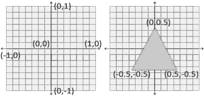
In order to draw something to begin with, we need to pass the vertex data to OpenGL. OpenGL is a 3D library and therefore all coordinates that we report to OpenGL are in three-dimensional space (x, y and z). OpenGL does not convert all 3D coordinates transferred to it to 2D pixels on the screen; OpenGL only processes 3D coordinates in a certain interval between -1.0 and 1.0 for all 3 coordinates (x, y and z). All such coordinates are called coordinates, normalized by the device (or simply normalized).

Since we want to draw one triangle, we must provide 3 vertices, each of which is in three-dimensional space. We define them in normalized form in the GLfloat array.

GLfloat vertices[] = { -0.5f, -0.5f, 0.0f, 0.5f, -0.5f, 0.0f, 0.0f, 0.5f, 0.0f }; 

Since OpenGL works with three-dimensional space, we draw a two-dimensional triangle with a z coordinate equal to 0.0. Thus, the depth of the triangle will be the same and it will look two-dimensional.

Normalized Device Coordinates (NDC)
After the vertex coordinates are processed in the vertex shader, they should be normalized to NDC, which is a small space where the x, y and z coordinates are in the range from -1.0 to 1.0 . Any coordinates that go beyond this limit will be dropped and not displayed on the screen. Below you can see the triangle defined by us:



Unlike the screen coordinates, the positive value of the y axis points to the top, and the coordinates (0, 0) is the center of the graph, instead of the upper left corner.

Your NDC coordinates will then be converted to screen space coordinates via Viewport using the data provided via the glViewport call. The coordinates of the screen space are then transformed into fragments and fed to the input of the fragment shader.

After determining the vertex data, it is required to transfer them to the first stage of the graphics pipeline: to the vertex shader. This is done as follows: allocate memory on the GPU, where we will save our vertex data, specify OpenGL how it should interpret the data transferred to it and transfer the amount of the data transferred by us to the GPU. Then the vertex shader will process the number of vertices that we told it.

We manage this memory through so-called vertex buffer objects (vertex buffer objects (VBO)), which can store a large number of vertices in the GPU memory. The advantage of using such buffer objects is that we can send a large number of data sets to a video card at a time, without having to send one vertex at a time. Sending data from the CPU to the GPU is rather slow, so we will try to send as much data as possible at a time. But as soon as the data is in the GPU, the vertex shader will get it almost instantly.

VBO is our first encounter with the objects described in the first lesson. Like any object in OpenGL, this buffer has a unique identifier. We can create a VBO using the glGenBuffers function:

 GLuint VBO; glGenBuffers(1, &VBO); 

OpenGL has a large number of different types of buffer objects. VBO type - GL_ARRAY_BUFFER . OpenGL allows you to bind multiple buffers if they have different types. We can bind GL_ARRAY_BUFFER to our buffer using glBindBuffer :

 glBindBuffer(GL_ARRAY_BUFFER, VBO); 

From now on, any call using the buffer will work with VBO. Now we can call glBufferData to copy the vertex data to this buffer.

 glBufferData(GL_ARRAY_BUFFER, sizeof(vertices), vertices, GL_STATIC_DRAW); 

glBufferData is a function whose purpose is to copy user data to the specified buffer. Its first argument is the type of buffer to which we want to copy data (our VBO is now bound to GL_ARRAY_BUFFER ). The second argument specifies the amount of data (in bytes) that we want to transfer to the buffer. The third argument is the data itself.

The fourth argument determines how we want the video card to work with the data passed to it. There are 3 modes:

1. GL_STATIC_DRAW : either the data will never change or will change very rarely;
2. GL_DYNAMIC_DRAW : data will change quite often;
3. GL_STREAM_DRAW : data will change with each drawing.

Triangle position data will not change and therefore we select GL_STATIC_DRAW . If, for example, we would have a buffer, the value of which would change very often - then we would use GL_DYNAMIC_DRAW or GL_STREAM_DRAW , thus providing the video card with the information that the data of this buffer needs to be stored in the memory area that is the fastest to write.

We have now saved the vertex data on the GPU to a buffer object called a VBO.
Next we need to create vertex and fragment shaders for actual data processing, so let's start.

Vertex shader

The vertex shader is one of the programmable shaders. Modern OpenGL requires that a vertex and fragment shaders be specified if we want to draw something, so we will provide two very simple shaders to draw our triangle. In the next lesson, we will discuss shaders in more detail.

In the beginning, we have to write the shader itself in a special GLSL (OpenGL Shading Language) language, and then compile it so that the application can work with it. Here is the simplest shader code:

 #version 330 core layout (location = 0) in vec3 position; void main() { gl_Position = vec4(position.x, position.y, position.z, 1.0); } 

As you can see, GLSL is very similar to C. Each shader begins with the installation of its version. With OpenGL version 3.3 and higher, the GLSL versions are the same as the OpenGL versions (For example, the GLSL 420 version is the same as the OpenGL version 4.2). We also clearly indicated that we are using the core profile.

Next, we specified all input vertex attributes in the vertex shader using the in keyword. Now we need to work only with position data, so we specify only one vertex attribute. In GLSL, there is a vector data type containing from 1 to 4 floating point numbers. Since the vertices have three-dimensional coordinates, we create a vec3 with the name position . We also explicitly specified the position of our variable through the layout (location = 0) later you will see why we did it.

Vector
In graphic programming, we quite often use the mathematical concept of a vector, since it perfectly represents positions / directions in any space, and also has useful mathematical properties. The maximum size of a vector in GLSL is 4 elements, and access to each of the elements can be obtained through vec.x , vec.y , vec.z and vec.w respectively. Notice that the vec.w component is not used as a position in space (we work in 3D, not in 4D), but it can be useful when working with perspective division. We will discuss vectors more deeply in the next lesson.

To indicate the result of the vertex shader, we must assign the value of the predefined variable gl_Position , which is of type vec4 . After the end of the main function, no matter what we pass to gl_Position, it will be used as the result of the vertex shader. Since our input vector is three-dimensional, we must convert it to four-dimensional. We can do this simply by passing the vec3 components to vec4 , and setting the w component to the value 1.0f (We will explain why so later).

This vertex shader is probably the easiest shader you can think of, since it does not process any data, but simply passes this data to the output. In real-world applications, the input data is not normalized, so at the beginning they need to be normalized.

Shader build

We wrote the shader source code (stored in the C string), but in order for the shaders to use OpenGL, it needs to be compiled.

In the beginning, we need to create a shader object. And since access to the created objects is done through the identifier, we will store it in a variable with the GLuint type, and we will create it through glCreateShader :

 GLuint vertexShader; vertexShader = glCreateShader(GL_VERTEX_SHADER); 

During the creation of the shader, we must specify the type of shader to create. Since we need a vertex shader, we specify GL_VERTEX_SHADER .

Next, we bind the shader source code to the shader object and compile it.

 glShaderSource(vertexShader, 1, &vertexShaderSource, NULL); glCompileShader(vertexShader); 

The glShaderSource function takes as its first argument a shader that needs to be built. The second argument describes the number of lines. In our case, the line is only one. The third parameter is the shader source code itself, and the fourth parameter is left in NULL.

Most likely you will want to check the success of the shader assembly. And if the shader was not compiled - get errors that occurred during the build. Check for errors is as follows:

 GLint success; GLchar infoLog[512]; glGetShaderiv(vertexShader, GL_COMPILE_STATUS, &success); 

To begin with, we declare a number to determine the success of the assembly and a container for storing errors (if they appear). We then test success with glGetShaderiv . If the build fails, then we will be able to get an error message with glGetShaderInfoLog and output this error:

 if(!success) { glGetShaderInfoLog(vertexShader, 512, NULL, infoLog); std::cout << "ERROR::SHADER::VERTEX::COMPILATION_FAILED\n" << infoLog << std::endl; } 

After that, if no compilation errors occurred - the shader will be compiled.

Fragment Shader

The fragment shader is the second and last shader that we need to draw a triangle. The fragment shader is responsible for calculating pixel colors. In the name of simplicity, our fragment shader will display only orange color.

Color in computer graphics is represented as an array of 4 values: red, green, blue and transparency; Such component base is called RGBA. When we set a color in OpenGL or in GLSL we set the size of each component between 0.0 and 1.0. If, for example, we set the magnitude of the red and green components to 1.0f, then we get a mixture of these colors — yellow. The combination of 3 components gives about 16 million different colors.

 #version 330 core out vec4 color; void main() { color = vec4(1.0f, 0.5f, 0.2f, 1.0f); } 

The fragment shader output requires only a color value, which is the 4 component vector. We can specify the output variable using the out keyword, and we call this variable color . Then we simply set the value of this variable to vec4 with an opaque orange color.

The process of assembling a fragmentary shader is similar to that of a vertex one, it is only necessary to specify a different type of shader: GL_FRAGMENT_SHADER :

 GLuint fragmentShader; fragmentShader = glCreateShader(GL_FRAGMENT_SHADER); glShaderSource(fragmentShader, 1, &fragmentShaderSource, NULL); glCompileShader(fragmentShader); 

Both shaders were assembled and now it only remains to link them into the program so that we can use them when drawing.

Shader program

A shader program is an object that is the final result of a combination of several shaders. In order to use the assembled shaders, you need to connect them into an object of a shader program, and then activate this program when rendering objects, and this program will be used when invoking the draw commands.

When connecting shaders to a program, the output values ​​of one shader are matched with the input values ​​of another shader. You can also get errors during the connection of shaders, if the input and output values ​​do not match.

Creating a program is very simple:

 GLuint shaderProgram; shaderProgram = glCreateProgram(); 

The glCreateProgram function creates a program and returns the ID of this program. Now we need to attach our assembled shaders to the program, and then link them with the glLinkProgram :

 glAttachShader(shaderProgram, vertexShader); glAttachShader(shaderProgram, fragmentShader); glLinkProgram(shaderProgram); 

This code completely describes itself. We add shaders to the program, and then link them.

As with the shader build, we can get a successful binding and an error message. The only difference is that instead of glGetShaderiv and glGetShaderInfoLog we use:

 glGetProgramiv(shaderProgram, GL_LINK_STATUS, &success); If (!success) { glGetProgramInfoLog(shaderProgram, 512, NULL, infoLog); … } 

To use the created program, call glUseProgram :

 glUseProgram(shaderProgram); 

Each call to the shader and drawing functions will use our program object (and, accordingly, our shaders).

Oh yes, do not forget to delete the created shaders after binding. We will not need them anymore.

 glDeleteShader(vertexShader); glDeleteShader(fragmentShader); 

At this point, we passed the vertex data to the GPU and told the GPU how to process it. We are almost done. OpenGL still doesn’t know how to present vertex data in memory and how to merge vertex data into vertex shader attributes. Well, let's get started.

Vertex attribute binding

The vertex shader allows us to specify any data in each vertex attribute, but this does not mean that we will have to specify which data element belongs to which attribute. This means that we need to tell OpenGL to interpret the vertex data before rendering.

The format of our vertex buffer is as follows:

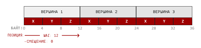
• Position information is stored in a 32 bit (4 byte) floating point value;
• Each position is formed from 3 values;
• There is no separator between sets of 3 values. This buffer is called tightly packed ;
• The first value in the transmitted data is the beginning of the buffer.

Knowing these features, we can tell OpenGL how it should interpret the vertex data. This is done using the glVertexAttribPointer function:

 glVertexAttribPointer(0, 3, GL_FLOAT, GL_FALSE, 3 * sizeof(GLfloat), (GLvoid*)0); glEnableVertexAttribArray(0); 

The glVertexAttribPointer function has some parameters, let's quickly run through them:

• The first argument describes which shader argument we want to configure. We want to specify the value of the position argument, the position of which was specified as follows: layout (location = 0).
  
  
• The following argument describes the size of the argument in the shader. Since we used vec3, we specify 3.
  
  
• The third argument describes the data type used. We specify GL_FLOAT , because vec in the shader uses floating point numbers.
  
  
• The fourth argument indicates the need to normalize the input data. If we specify GL_TRUE , then all data will be located between 0 (-1 for character values) and 1. We do not need normalization, so we leave GL_FALSE ;
  
  
• The fifth argument is called step and describes the distance between the data sets. We can also specify a step equal to 0 and then OpenGL will calculate the step (works only with tightly packed data sets). How to gain substantial benefits from this argument, we will look at later.
  
  
• The last parameter is of type GLvoid * and therefore requires such a strange type conversion. This is the offset of the beginning of the data in the buffer. Our buffer has no offset and therefore we specify 0.

Each vertex attribute gets a value from VBO-managed memory that is currently bound to GL_ARRAY_BUFFER . Accordingly, if we called glVertexAttribPointer with another VBO, then the vertex data would be taken from another VBO.

After we tell OpenGL how it should interpret the vertex data, we need to include the attribute with glEnableVertexAttribArray . Thus, we will pass the position of the argument to the vertex attribute. After we set everything up, we initialized the vertex data in the buffer using VBO, installed the vertex and fragment shader, and told OpenGL how to link the vertex shader and the vertex data. Drawing an object in OpenGL will look something like this:

 // 0.       OpenGL glBindBuffer(GL_ARRAY_BUFFER, VBO); glBufferData(GL_ARRAY_BUFFER, sizeof(vertices), vertices, GL_STATIC_DRAW); // 1.       glVertexAttribPointer(0, 3, GL_FLOAT, GL_FALSE, 3 * sizeof(GLfloat), (GLvoid*)0); // 2.     glUseProgram(shaderProgram); // 3.     someOpenGlFunctionThatDrawsOutTriangle(); 

We must repeat this process every time we draw an object. It seems that this is not very difficult, but now imagine that you have more than 5 vertex attributes and something in the region of 100 different objects. And immediately the constant installation of these configurations for each object becomes a wild routine. That would be some way to store all these states and that we would only need to be attached to some state to draw ...

Vertex Array Object

A vertex array object (VAO) can also be bound as a VBO and after that all subsequent calls to the vertex attributes will be stored in the VAO. The advantage of this method is that we only need to configure the attributes once, and all subsequent times the VAO configuration will be used. Also, this method makes it easy to change vertex data and attribute configurations by simply binding different VAOs.

Core OpenGL requires that we use VAO in order for OpenGL to know how to work with our input vertices. If we do not specify a VAO, OpenGL may refuse to draw anything.

VAO stores the following calls:

• Calls glEnableVertexAttribArray or glDisableVertexAttribArray .
• Attribute configuration via glVertexAttribPointer .
• VBO associated with vertex attributes using glVertexAttribPointer

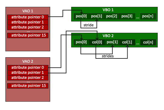
The VAO generation process is very similar to the VBO generation:

 GLuint VAO; glGenVertexArrays(1, &VAO); 

In order to use VAO, all you have to do is bind the VAO with glBindVertexArray . Now we have to adjust / bind the required VBO and attribute pointers, and at the end untie the VAO for later use. And now, every time when we want to draw an object, we simply bind the VAO with the required settings before drawing the object. It all should look something like this:

 // ..::   (  (, ,     )) :: .. // 1.  VAO glBindVertexArray(VAO); // 2.        OpenGL glBindBuffer(GL_ARRAY_BUFFER, VBO); glBufferData(GL_ARRAY_BUFFER, sizeof(vertices), vertices, GL_STATIC_DRAW); // 3.      glVertexAttribPointer(0, 3, GL_FLOAT, GL_FALSE, 3 * sizeof(GLfloat), (GLvoid*)0); glEnableVertexAttribArray(0); //4.  VAO glBindVertexArray(0); [...] // ..::   (  ) :: .. // 5.   glUseProgram(shaderProgram); glBindVertexArray(VAO); someOpenGLFunctionThatDrawsOurTriangle(); glBindVertexArray(0); 

Unlocking objects in OpenGL is common. At least just to not accidentally spoil the configuration.

That's all! Everything we have done over millions of pages has brought us to this point. VAO storing vertex attributes and required VBO. Often, when we have multiple objects to render, we first generate and configure VAO and save them for later use. And when we need to draw one of our objects, we simply use the saved VAO.

The triangle we were waiting for

To render our objects, OpenGL provides us with the glDrawArrays function. It uses the active shader and the installed VAO to render the specified primitives.

 glUseProgram(shaderProgram); glBindVertexArray(VAO); glDrawArrays(GL_TRIANGLES, 0, 3); glBindVertexArray(0); 

The glDrawArrays function takes the primitive to be drawn as the first argument of OpenGL. Since we want to draw a triangle and since we do not want to lie to you, we specify GL_TRIANGLES . , , 0. , 3 ( — 3 ).

. :



.

, , - . .

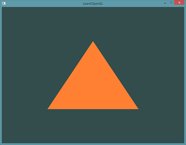
Element Buffer Object

The last thing we’ll talk about today on vertex drawing is element buffer objects (EBO). In order to explain what this is and how it works it is better to give an example: suppose that we need to draw not a triangle, but a quadrilateral. We can draw a quad with 2 triangles (OpenGL basically works with triangles).

A note from the translator.
As noted by the proydakov user , this object is also called the Index Buffer Object, respectively IBO.

Accordingly, it will be necessary to declare the following set of vertices:

 GLfloat vertices[] = { //   0.5f, 0.5f, 0.0f, //    0.5f, -0.5f, 0.0f, //    -0.5f, 0.5f, 0.0f, //    //   0.5f, -0.5f, 0.0f, //    -0.5f, -0.5f, 0.0f, //    -0.5f, 0.5f, 0.0f //    }; 

: . , 4 6. , 1000 . — , . 4 , . , OpenGL .

EBO , . EBO — , VBO, , OpenGL , . (indexed drawing) . :

 GLfloat vertices[] = { 0.5f, 0.5f, 0.0f, //    0.5f, -0.5f, 0.0f, //    -0.5f, -0.5f, 0.0f, //    -0.5f, 0.5f, 0.0f //    }; GLuint indices[] = { // ,     0! 0, 1, 3, //   1, 2, 3 //   }; 

, 4 6. EBO:

 GLuint EBO; glGenBuffers(1, &EBO); 

VBO EBO glBufferData . , VBO ( glBindBuffer(GL_ELEMENT_ARRAY_BUFFER, 0) , GL_ELEMENT_ARRAY_BUFFER .

 glBindBuffer(GL_ELEMENT_ARRAY_BUFFER, EBO); glBufferData(GL_ELEMENT_ARRAY_BUFFER, sizeof(indices), indices, GL_STATIC_DRAW); 

, GL_ELEMENT_ARRAY_BUFFER . — glDrawArrays glDrawElements , , . glDrawElements EBO:

 glBindBuffer(GL_ELEMENT_ARRAY_BUFFER, EBO); glDrawElements(GL_TRIANGLES, 6, GL_UNSIGNED_INT, 0); 

, , glDrawArrays . — , . 6 , 6 . — , — GL_UNSIGNED_INT . EBO ( , EBO ), 0.

glDrawElements GL_ELEMENT_ARRAY_BUFFER EBO. , EBO. VAO EBO.

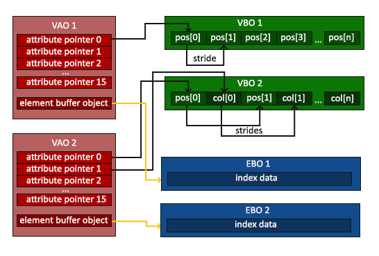
VAO glBindBuffer, GL_ELEMENT_ARRAY_BUFFER. , , , EBO VAO, EBO.

:

 // ..::   :: .. // 1.  VAO glBindVertexArray(VAO); // 2.       OpenGL glBindBuffer(GL_ARRAY_BUFFER, VBO); glBufferData(GL_ARRAY_BUFFER, sizeof(vertices), vertices, GL_STATIC_DRAW); // 3.        OpenGL glBindBuffer(GL_ELEMENT_ARRAY_BUFFER, EBO); glBufferData(GL_ELEMENT_ARRAY_BUFFER, sizeof(indices), indices, GL_STATIC_DRAW); // 3.      glVertexAttribPointer(0, 3, GL_FLOAT, GL_FALSE, 3 * sizeof(GLfloat), (GLvoid*)0); glEnableVertexAttribArray(0); // 4.  VAO ( EBO) glBindVertexArray(0); [...] // ..::   (  ) :: .. glUseProgram(shaderProgram); glBindVertexArray(VAO); glDrawElements(GL_TRIANGLES, 6, GL_UNSIGNED_INT, 0) glBindVertexArray(0); 

. , — wireframe. 2 .

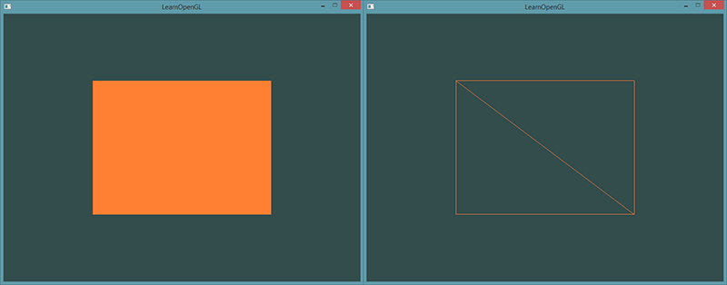
Wireframe

, OpenGL, glPolygonMode(GL_FRONT_AND_BACK, GL_LINE) . , , , . , — glPolygonMode(GL_FRONT_AND_BACK, GL_FILL).

If you have any problems, go over the lesson, maybe you forgot something. You can also check with the source code .

If everything worked out for you, congratulations, you just went through one of the most difficult parts of studying modern OpenGL: the output of the first triangle. This part is so complex because it requires a certain amount of knowledge before it is possible to draw the first triangle. Fortunately, we have already gone through this and subsequent lessons should be easier.

Additional resources

• antongerdelan.net/hellotriangle : Anton Gerdelans draws the first triangle ..
• open.gl/drawing : Alexander Overvoordes draws the first triangle.
• antongerdelan.net/vertexbuffers : a small depression in the VBO.
• learnopengl.com/#!In-Practice/Debugging : In this lesson a lot has been taken from this lesson; if you are stuck somewhere, you can turn to this page. (After translating this page, I will link to the translation).

Exercises

To consolidate the studied I will propose several exercises:

1. Try drawing 2 triangles one by one using glDrawArrays by adding more vertices. Decision
2. Create 2 triangles using 2 different VAO and VBO. Decision
3. Create a second fragment shader so that it displays a yellow color. And make the second triangle be yellow. Decision