Overview of deep convolutional neural network topologies
 This will be a long post. I have long wanted to write this review, but I was ahead of sim0nsays , and I decided to wait a moment, for example, how the results of ImageNet will appear. Now the moment has come, but imajnet has not brought any surprises, except that Chinese efesbeshniki are in the first place by classification. Their model, in the best traditions of CGL, is an ensemble of several models (Inception, ResNet, Inception ResNet), and overtakes the past winners by only half a percent (by the way, there is no publication yet, and there is a miserable chance that there is really something new). By the way, as you can see from the results of imajnet, something went wrong with the addition of layers, as evidenced by the growth in the width of the architecture of the final model. Maybe from neural networks have already squeezed all that is possible? Or does NVidia raise the price of the GPU too much and thus slows down the development of AI? Is winter close? In general, I will not answer these questions here. But under the cut you will find a lot of pictures, layers and dances with a tambourine. It is implied that you are already familiar with the error back-propagation algorithm and understand how the basic building blocks of convolutional neural networks work: convolutions and pooling.
The transition from neurophysiology to computer vision
 The story should have been started with the pioneers of neural networks (not only artificial) and their contribution: the McCulloch-Pitts formal neuron model, Hebb’s learning theory , Rosenblatt perceptron , Paul Bach-Rita’s experiments and others, but I’ll leave it to readers for independent work. So I propose to go straight to David Hubel and Torsten Wiesel, the Nobel laureates of 1981. They received an award for work carried out in 1959 (at the same time, Rosenblatt put his experiments). Formally, the prize was awarded for "work concerning the principles of information processing in neural structures and mechanisms of brain activity." It is necessary to immediately warn sensitive readers: then an experiment with cats will be described. The model of the experiment is depicted in the figure below: a bright elongated moving rectangle is shown to the cat on a dark screen at various angles; The oscilloscope electrode is connected to the occipital part of the brain, where mammals have a visual information processing center. In the course of the experiment, scientists observed the following effects (you can easily find analogies with modern convolutional networks and recurrent networks):
')
- certain areas of the visual cortex are activated only when the line is projected onto a certain part of the retina;
- the level of activity of the neurons in the area changes as the angle of inclination of the rectangle changes;
- Some areas are activated only when the object moves in a certain direction.
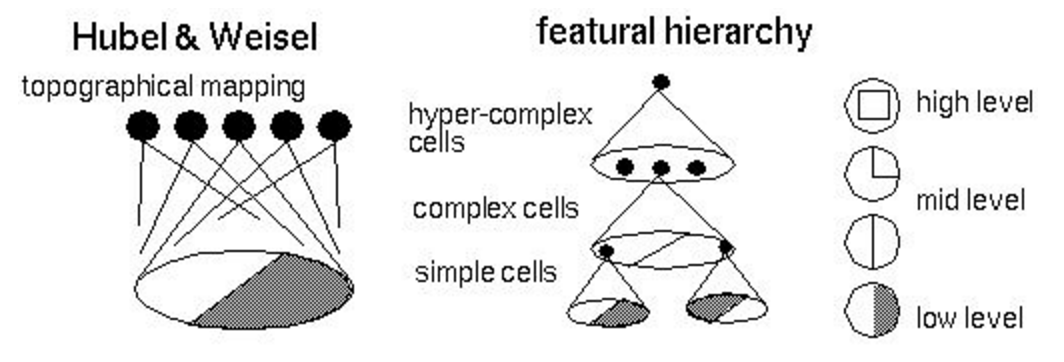
One of the results of the study was a model of the visual system, or topographic map, with the following properties:
- neighboring neurons process signals from neighboring areas of the retina;
- neurons form a hierarchical structure (image below), where each next level highlights more and more high-level signs (today we already know how to effectively manipulate these signs );
- neurons are organized into so-called columns - computational blocks that transform and transmit information from level to level.
The first who tried to put the ideas of Hubel and Wiesel into the program code was Kunihiko Fukushima, who offered two models from 1975 to 1980: the cognitron and the neocognitron . These models almost repeated the biological model , today we call simple cells (simple cells) convolutions , and complex cells (complex cells) pooling : these are still the basic building blocks of modern convolutional neural networks. The model was not taught by the error back-propagation algorithm, but by the original heuristic algorithm in the mode without a teacher. We can assume that this work was the beginning of neural network computer vision.
Document recognition (1998)
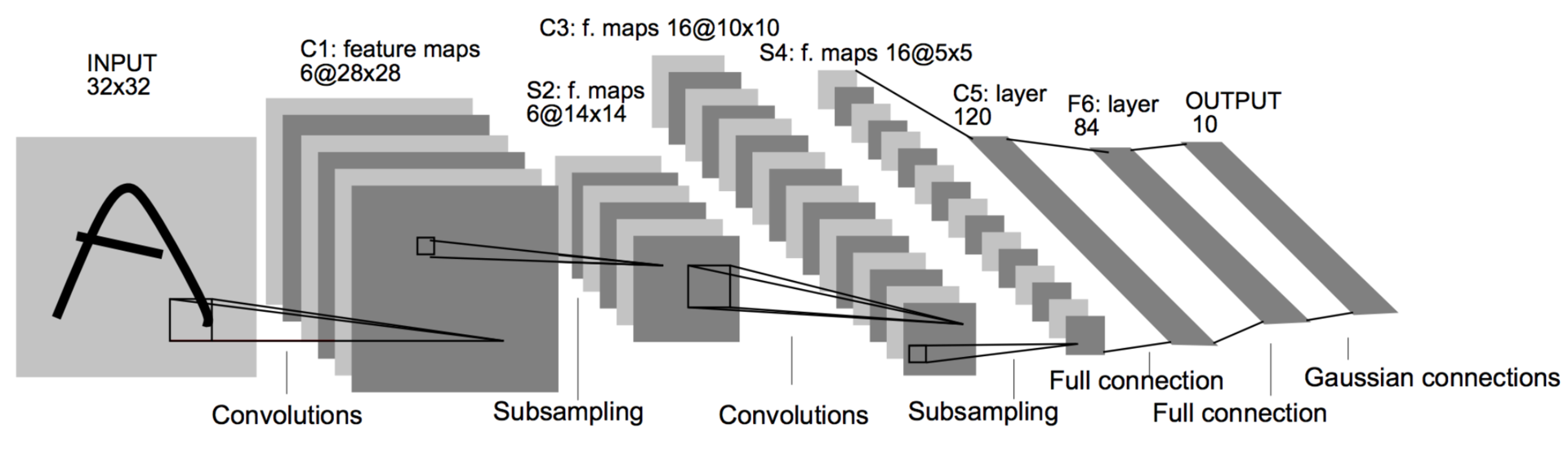
After many years, 1998 came. Winter has passed. Jan LeKunn , who has long been a postdoc of one of the authors of an article on the backpropagation algorithm, publishes a paper (in collaboration with other luminaries of neural networks), in which he mixes ideas of convolutions and pulling with backprop, eventually getting the first working convolutional neural network. It was introduced into the US mail for index recognition. This architecture was a standard template for building convolutional networks until recently: convolution alternates with pooling several times, then several fully connected layers. Such a network consists of 60 thousand parameters. The main building blocks are convolutions of 5 × 5 with a shift of 1 and 2 × 2 of shift with a shift of 2. As you already know, convolutions play the role of feature detectors, and pooling (or subsampling) is used to reduce the dimension by exploiting the fact that the images have the property local correlation of pixels - neighboring pixels, as a rule, do not differ much from each other. Thus, if you get any aggregate from several neighbors, then the loss of information will be insignificant.
ImageNet Classification with Deep Convolutional Neural Networks (2012)
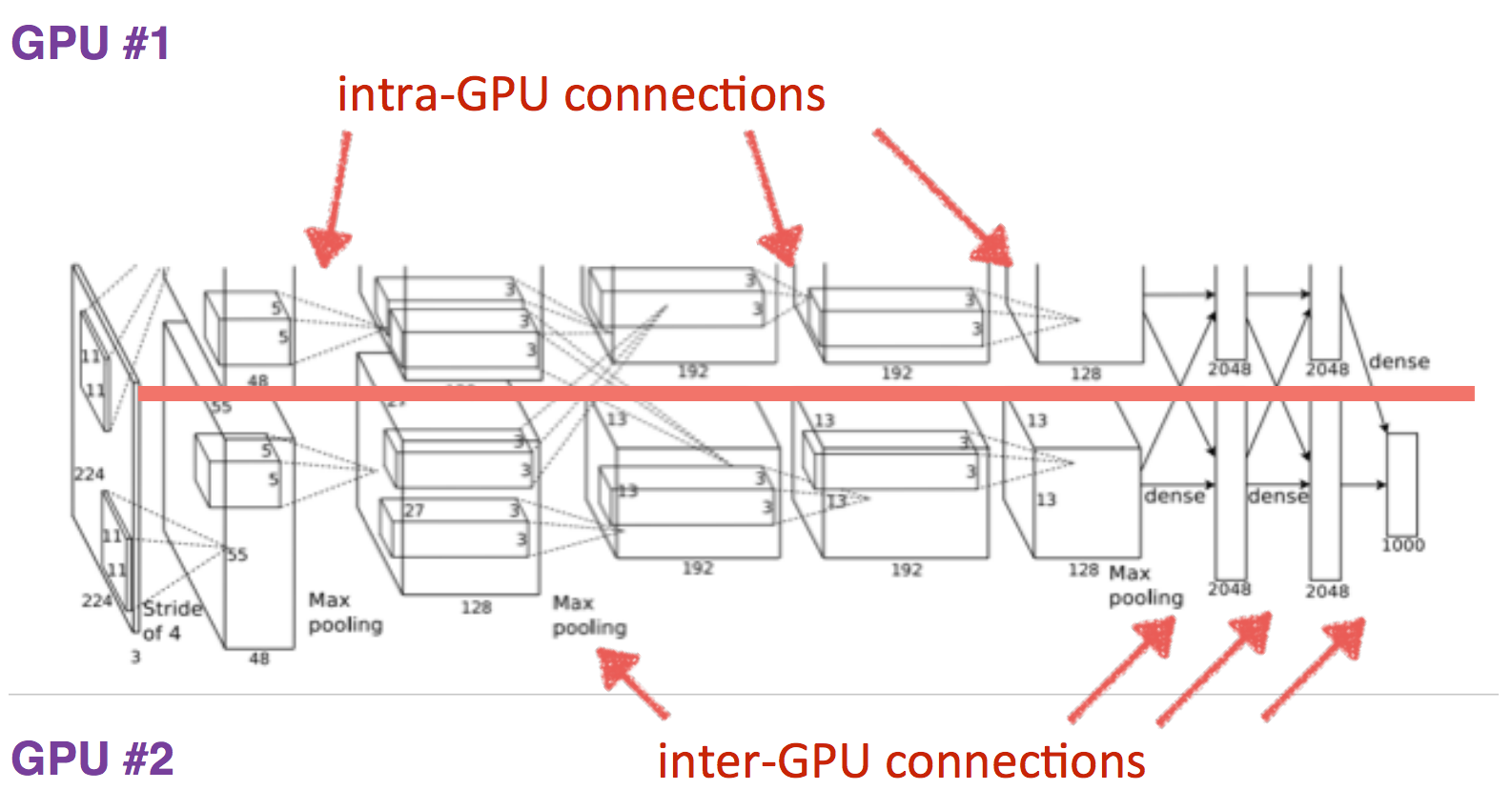
It took another 14 years. Alex Krizhevsky from the same laboratory where LeKun was a postdoc added the last ingredients to the formula. Deep learning = model + learning theory + big data + iron . GPU allowed to significantly increase the number of trained parameters. The model contains 60 million parameters, three orders of magnitude more; two graphic accelerators were used to train such a model.

Other images of AlexNet
Data exchange between GPUs
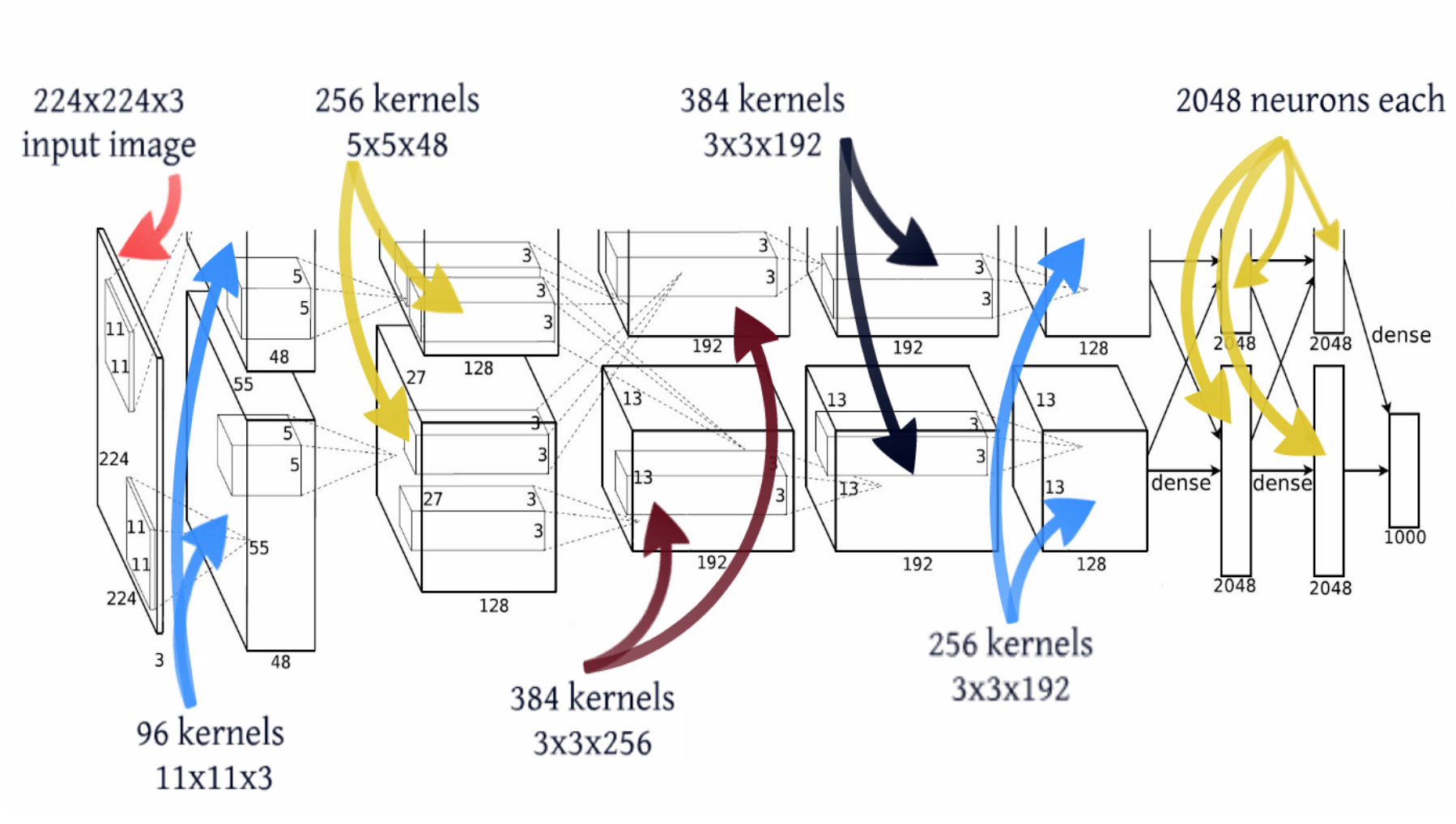
Sizes of layers
Sizes of layers
In terms of network topology, this is almost the same LeNet, just magnified a thousand times. Several more convolutional layers were added, and the size of the convolution kernels decreases from the input of the network to the output. This is explained by the fact that at the beginning the pixels are highly correlated, and the receptor area can be safely taken large, we still lose little information. Next, we apply pooling, thereby increasing the density of uncorrelated plots . At the next level, it is logical to take a slightly smaller receptor area. As a result, the authors turned out such a pyramid of bundles of 11 × 11 -> 5 × 5 -> 3 × 3 ...
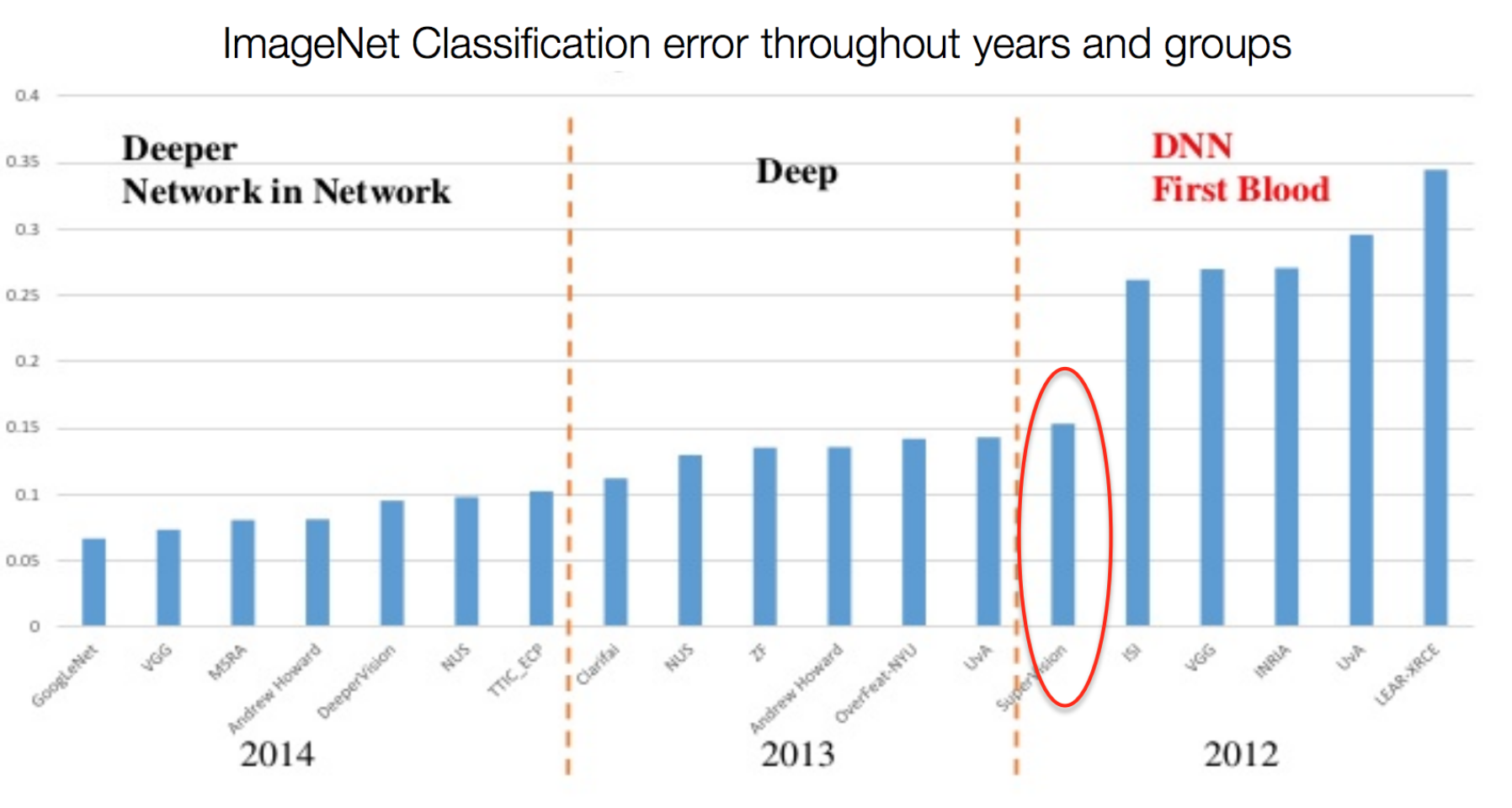
Other tricks have also been applied to avoid retraining, and some of them are now standard for deep networks: DropOut (RIP), Data Augmentation, and ReLu . We will not focus on these tricks, focus on the topology of the model. I will only add that since 2012, no neural network models have won the Imagnet anymore.
Very Deep Convolutional Networks for Large-Scale Image Recognition (12 Apr 2014)
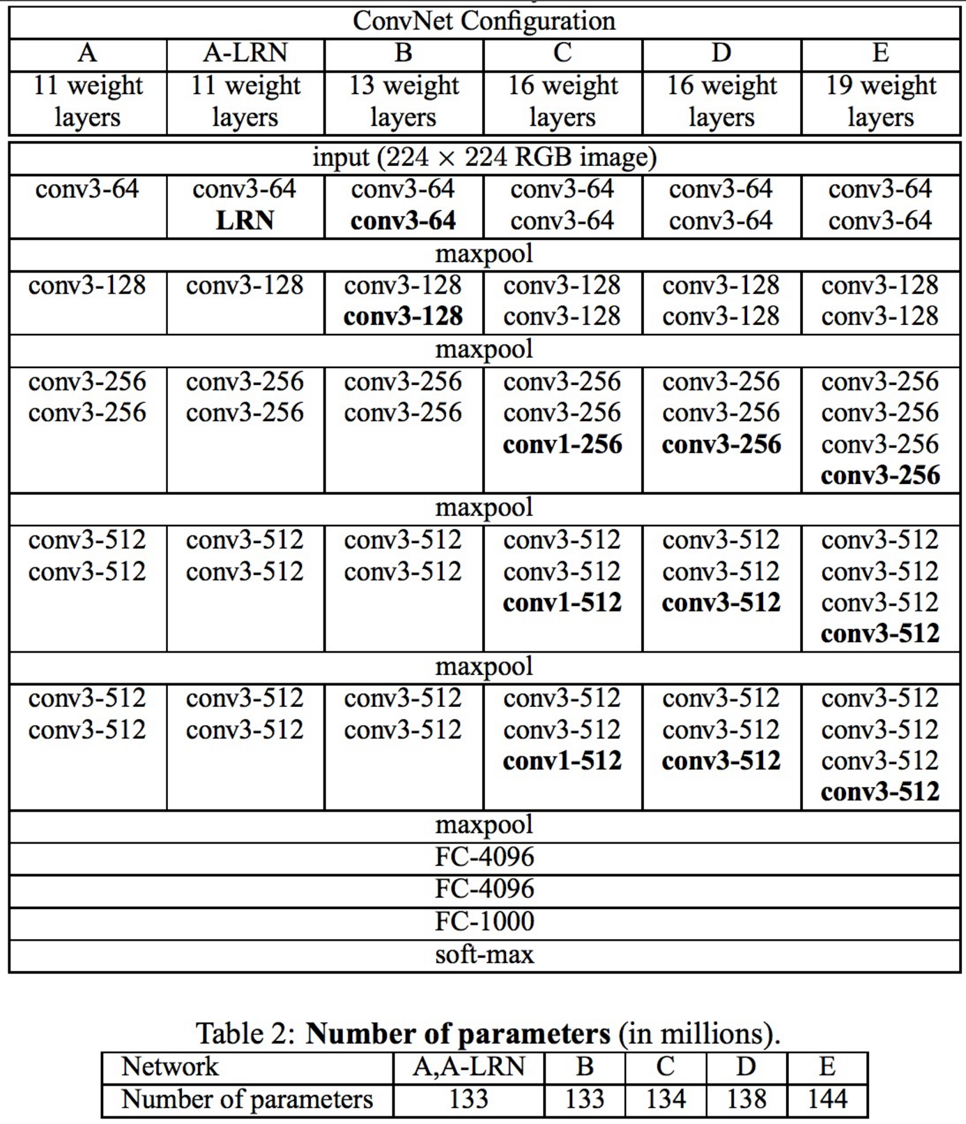
This year there were two interesting articles, this one and Google Inception, which we will discuss below. The work of the Oxford Laboratory is the last work adhering to the topology pattern laid down by LeCun. Their VGG-19 model consists of 144 million parameters and adds to the architecture, in addition to 84 million parameters, another simple idea. Take for example the convolution of 5 × 5, this mapping
 It contains 25 parameters. If we replace it with a stack of two layers with convolutions of 3 × 3, then we get the same display, but the number of parameters will be less: 3 × 3 + 3 × 3 = 18, which is 22% less. If we replace 11 × 11 by four 3 × 3 convolutions, then this is already 70% less than the parameters.
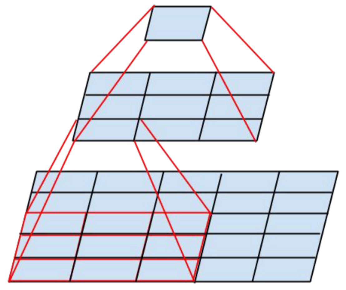
VGG- * Models
Network in Network (4 Mar 2014)
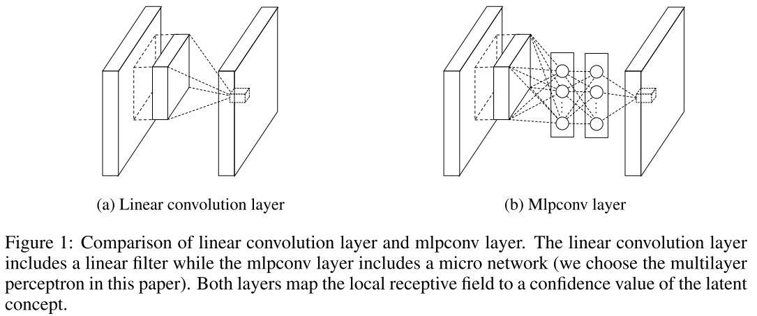
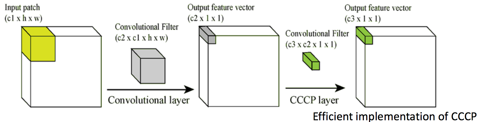
And here begin dancing with a tambourine. Such a picture was illustrated by the author of the publication of his blog post, where he spoke about ascaded ross han Channel Parameteric pooling. Consider the main ideas of this article. Obviously, the convolution operation is a linear transformation of the image patches, then the convolutional layer is a generalized linear model (GLM). It is assumed that the images are linearly separable. But why does CNN work? Everything is simple: a redundant representation is used (a large number of filters) to take into account all variations of one image in the feature space. The more filters on one layer, the more variations you need to take into account the next layer. What to do? Let's replace GLM with something more efficient, and the most effective one is the single-layer perceptron . This will allow us to more effectively divide the space of signs, thereby reducing their number.
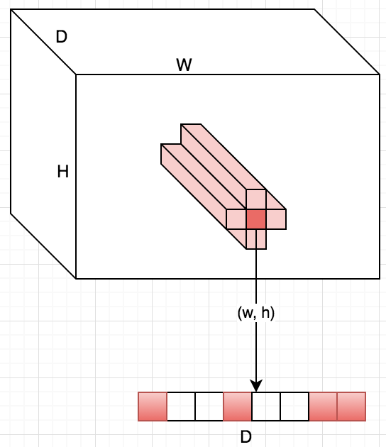
I am sure that you have already begun to doubt the expediency of such a decision, we will indeed reduce the number of signs, but significantly increase the number of parameters. The authors say that the USSR will solve this problem. It works as follows: at the exit of the convolutional layer, we get a cube of size W × H × D. For each position (w, h) take all the values on D, Cross Channel, and calculate the linear combination, Parametric pooling, and so we will do several times, thereby creating a new volume, and so several times - Cascade. It turns out that these are simply 1 × 1 convolutions with subsequent nonlinearity. This trick is ideologically the same as in the VGG article about 3 × 3 convolutions. It turns out that we first propose replacing ordinary convolution with MLP, but since MLP is very expensive, we replace every fully connected layer with a convolutional layer - this is a Singapore trick . It turns out that NIN is a deep convolutional neural network, and instead of convolutions there are small convolutional neural networks with a 1 × 1 core. In general, while they still did not know which genie they had released.
The next idea, even more interesting, is to completely abandon the fully connected layers - global average pooling. Such a network is called a fully convolutional network, since it no longer requires any specific image size to enter and consists only of bundles / pooling. Suppose there is a classification task into N classes, then instead of fully connected layers, a 1 × 1 convolution is used to make a W × H × N cube from the W × H × D cube, that is, the 1 × 1 convolution can be changed arbitrarily to the depth of the cube signs. When we have N W × H dies, we can calculate the average value of the dice and calculate softmax. A slightly deeper idea is contained in the authors' claim that earlier convolutional layers acted simply as mechanisms for extracting features, and discriminators were fully connected layers (from there such a pattern, given by LeCunn). The authors argue that convolutions are discriminators, too, since the network consists only of convolutions and solves the problem of classification. It is worth noting that in LeNet convolutional networks, 80% of the calculations are on convolutional layers, and 80% of memory consumption is on fully connected.
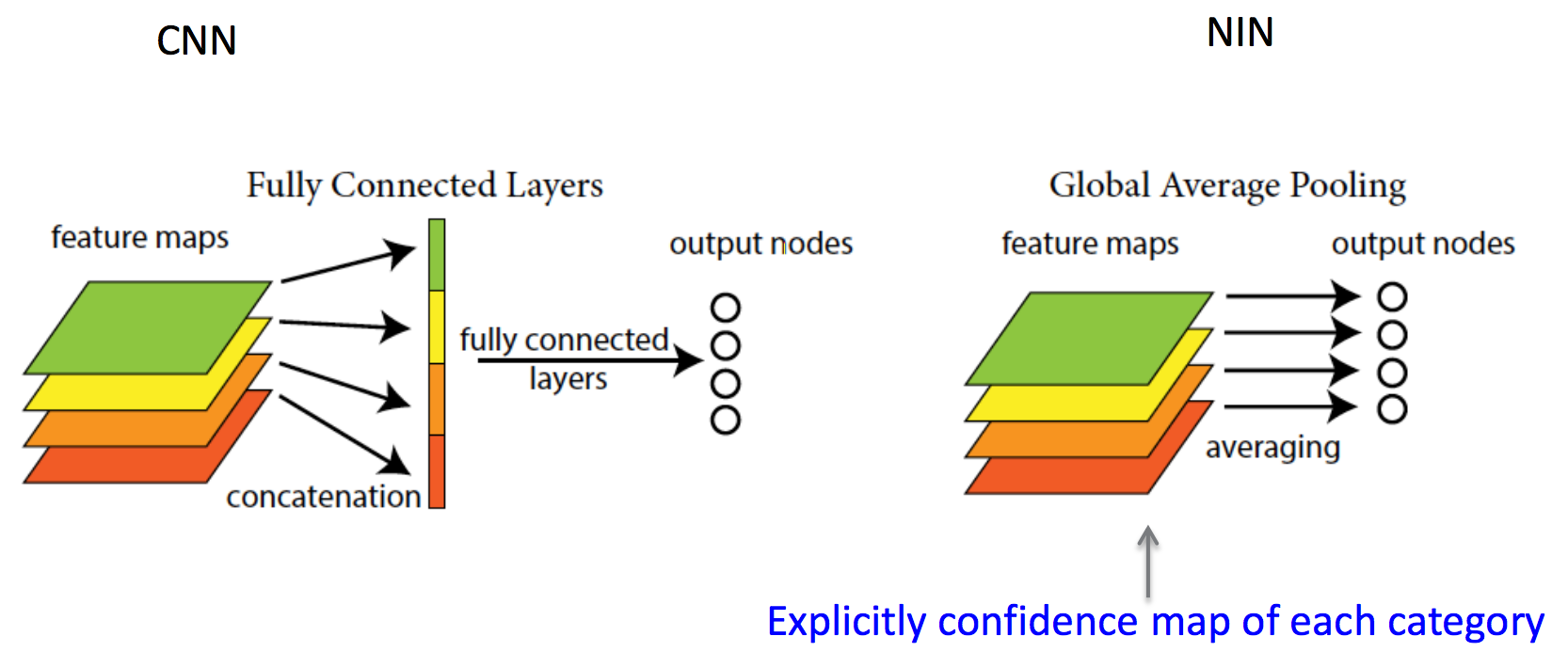
Later, LeKun will write on his Facebook:
In Convolutional Nets, there is no such thing as “fully-connected layers”. There are only convolution layers with 1 × 1 convolution kernels and a full connection table.
The only pity is that the authors who came up with so many new ideas did not participate in imagnet. On the other hand, Google jumped in on time and used these ideas in the next publication. As a result, Google shared the prizes in 2014 with a team from Oxford.
Going Deeper with Convolutions (17 Sep 2014)
Google comes into play, they called their network Inception, the name was not chosen by chance, it continues the ideas of previous work about the “Network within the Network”, as well as the well-known meme. Here is what the authors write:
In this paper, we’ve been able to follow the guidelines of the computer network. internet meme [1]. In the case of the “Inception module” depth. In general, it is possible to take a look at the theoretical work of Arora et al [2].
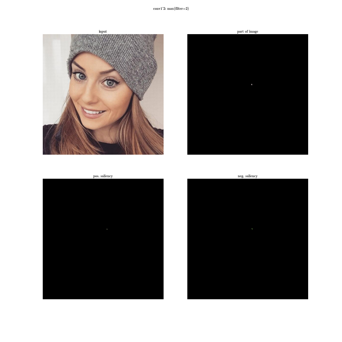
An arbitrary increase in the width (the number of neurons in the layers) and the depth (the number of layers) has several disadvantages. First, an increase in the number of parameters contributes to retraining, and an increase in the number of layers also adds to the problem of gradient decay. By the way, the last statement will be resolved by ResNet, which will be discussed further. Secondly, an increase in the number of convolutions in a layer leads to a quadratic increase in computations in this layer. If new model parameters are used inefficiently, for example, many of them become close to zero, then we just waste our computing power. Despite these problems, the first author of the article wanted to experiment with deep networks, but with a significantly smaller number of parameters. To do this, he turned to the article “ Provable Bounds for Learning Some Deep Representations ”, in which they prove that if the probabilistic distribution of data can be represented as a sparse, deep and wide neural network, then an optimal neural network can be constructed for a given dataset by analyzing the correlations of neurons the previous layer and combining the correlated neurons into groups that will be the neurons of the next layer. Thus, the neurons of the later layers "look" at the highly intersecting areas of the original image. Let me remind you how the receptor regions of neurons look at different levels and what signs they extract.
the receptor region of the layer conv1_2 of the network VGG-19
Yes, you see almost nothing, since the receptive area is very small, this is the second convolution 3 × 3, respectively, the general area is 5 × 5. But, having increased, we will see that the feature is just a gradient detector.
the receptor region of the conv3_3 layer of the VGG-19 network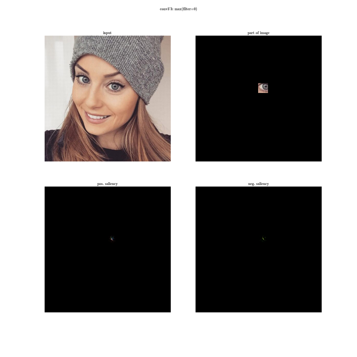
the receptor region of the conv4_3 layer of the VGG-19 network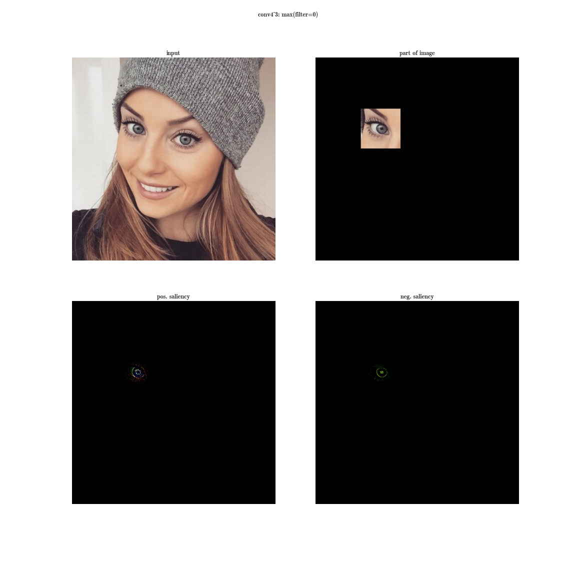
receptor region of the convG_3 layer of the VGG-19 network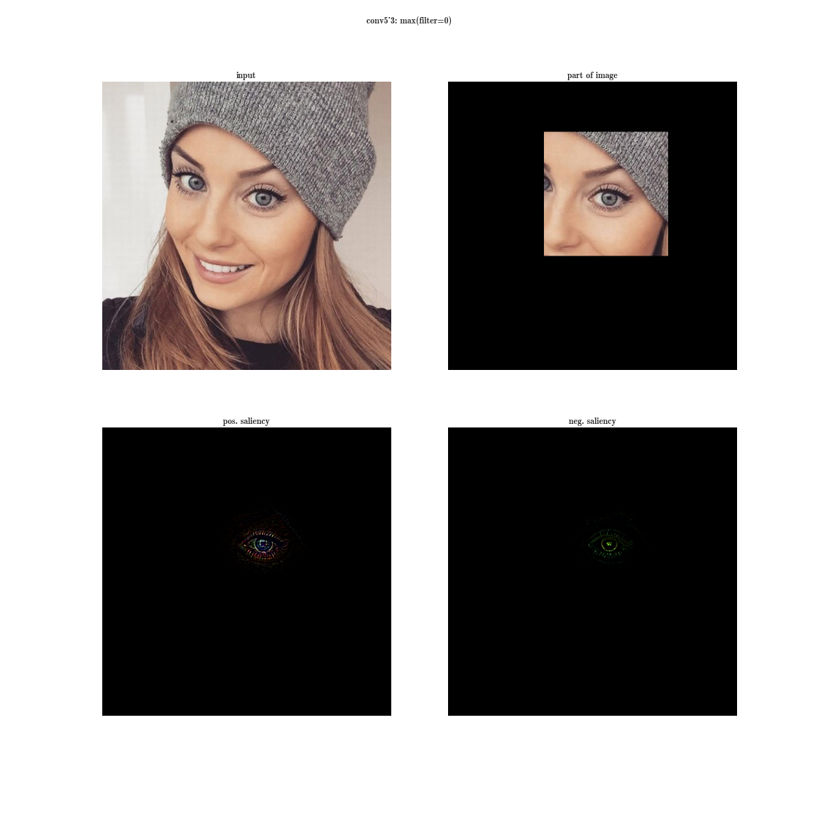
receptor region of the pool5 layer of the VGG-19 network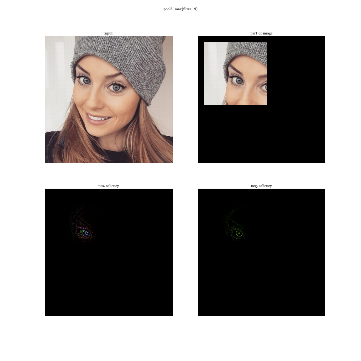
In the early layers (closer to the entrance), the correlated neurons will be concentrated in local areas. This means that if several neurons in one coordinate (w, h) on a plate can learn about the same thing, then in the tensor after the first layer of their activation they will be located in a small region at a certain point (w, h), and will be along the dimension of the filter bank - D. Like this:
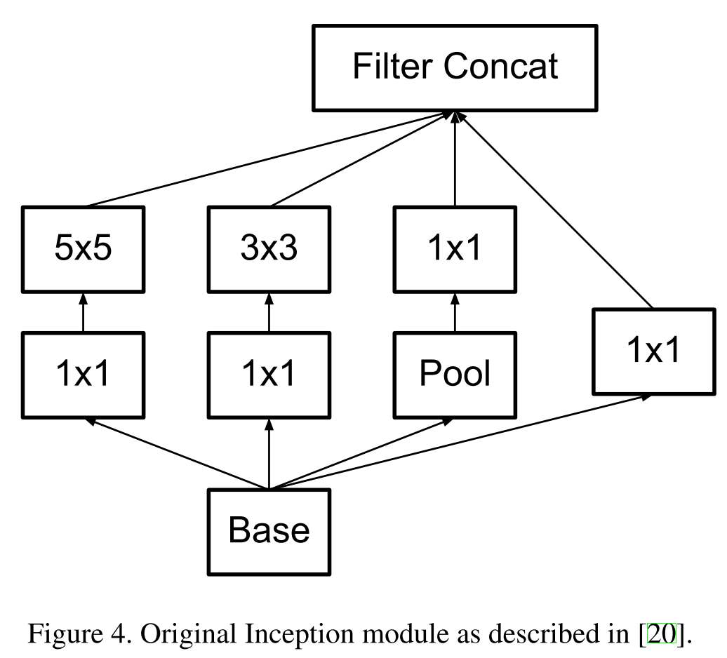
How, then, to catch such correlations and turn them into one sign? The idea of a 1 × 1 bundle from a previous paper comes to the rescue. Continuing this idea, it can be assumed that a slightly smaller number of correlated clusters will be slightly larger, for example, 3 × 3. The same is true for 5 × 5, etc., but Google decided to stop at 5 × 5.
convolutions 1 × 1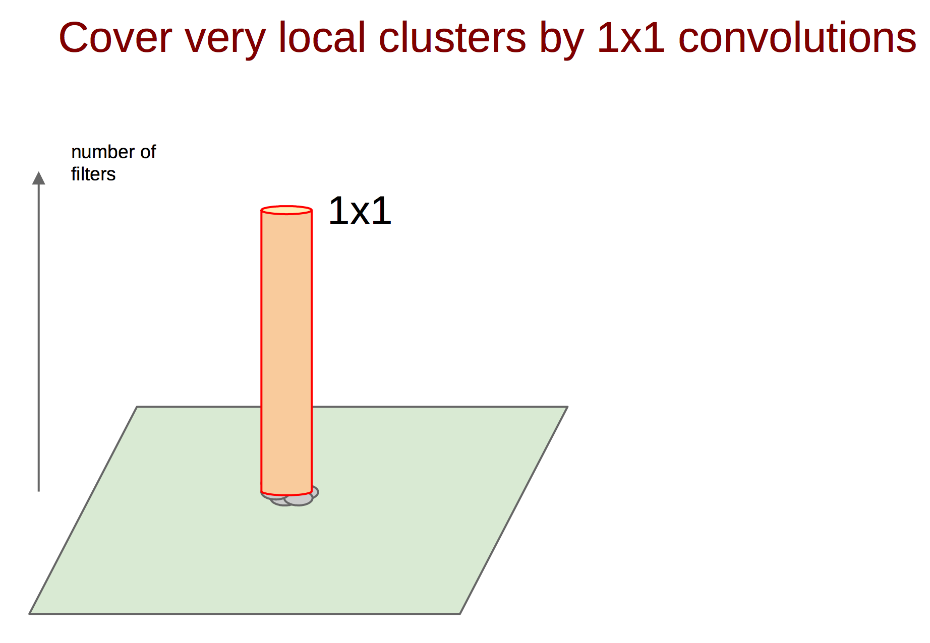
convolutions 3 × 3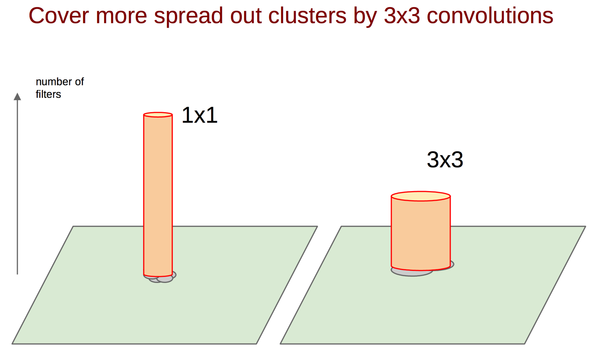
convolutions 5 × 5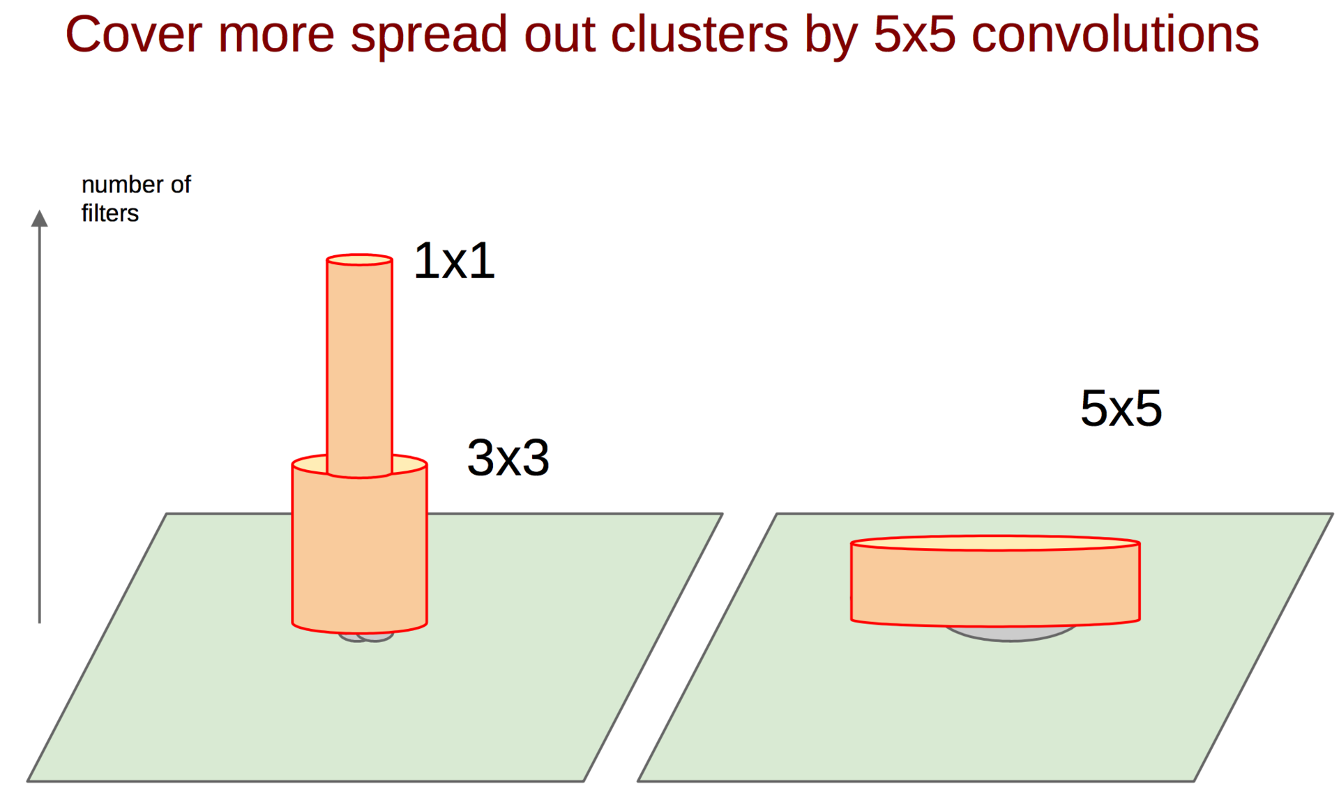
After calculating the feature maps for each convolution, it is necessary to aggregate them in some way, for example, to concatenate filters.
concatenation of signs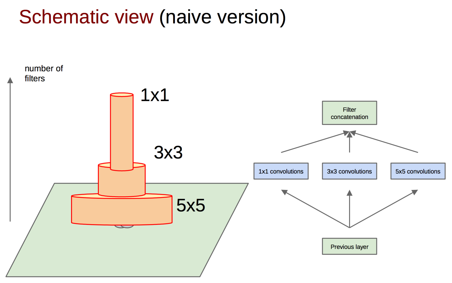
By the way, in order not to lose the original image from the previous layer, in addition to convolutions, pooling signs are added (we remember that the pooling operation does not entail large losses of information). Anyway, everybody uses pooling - there is no reason to refuse it. The whole group of several operations is called an Inception block.
In addition, since it’s not possible, then.
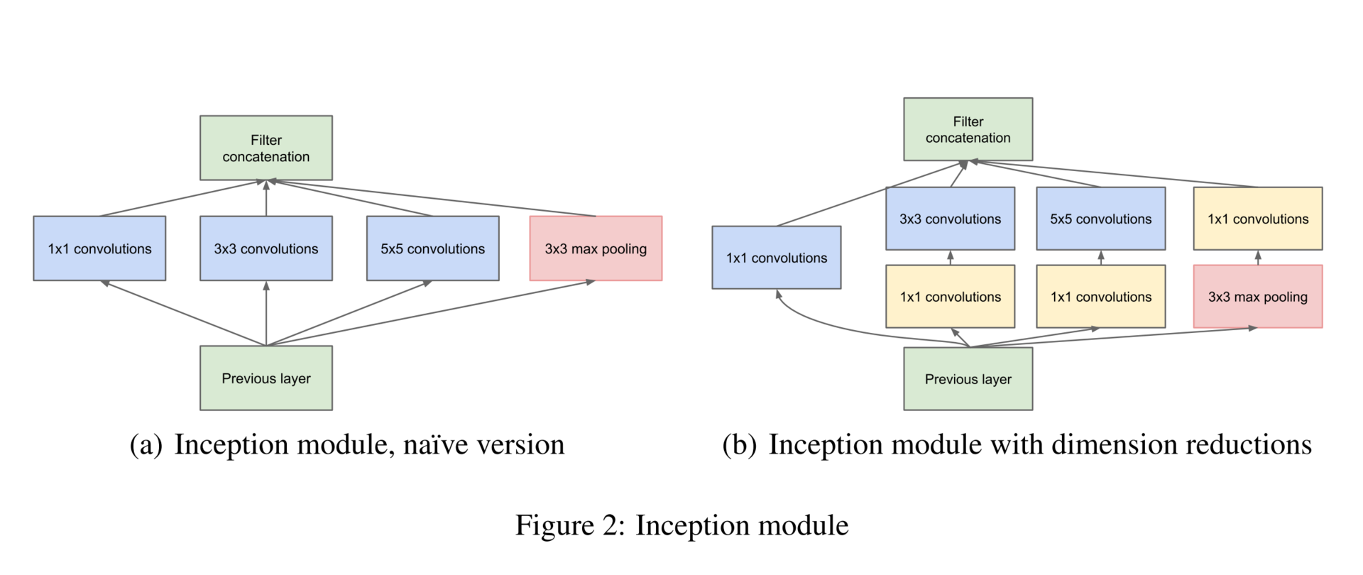
In order to equalize the size of the output tensors, it is also proposed to use a 1 × 1 convolution; In addition, 1 × 1 convolutions are also used to reduce the dimension before energy-consuming convolution operations. As you can see, Google uses 1 × 1 convolutions to achieve these goals (the next generation of networks will also exploit these techniques):
- increasing the dimension (after surgery);
- reduce the dimension (before the operation);
- grouping of correlated values (the first operation in the block).
The final model is as follows:
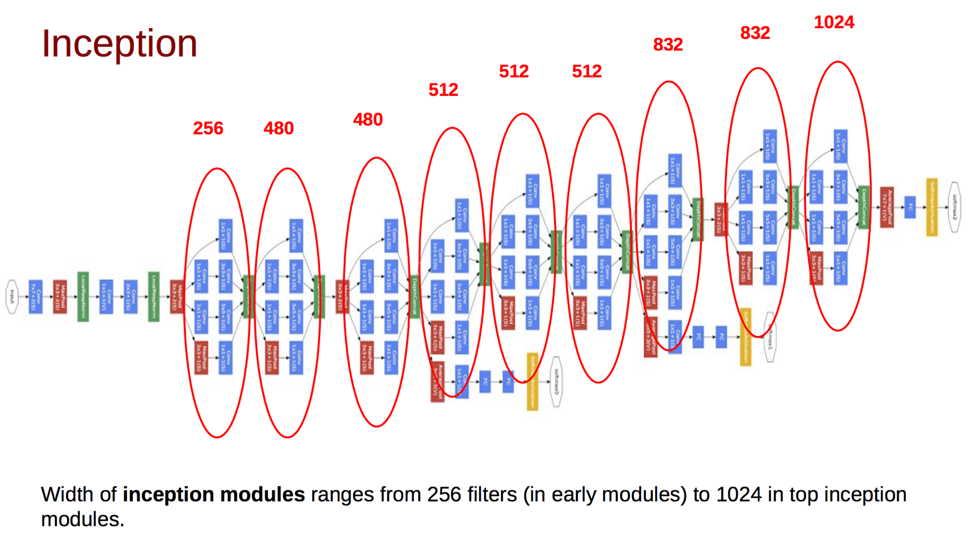
In addition to the above, you may notice several additional classifiers at different levels. The initial idea was that such classifiers would “push” the gradients to the early layers and thereby reduce the gradient damping effect. Later, Google will refuse them. The network itself gradually increases the depth of the tensor and reduces the spatial dimension. At the end of the article, the authors leave open the question of the effectiveness of such a model, and also hint that they will investigate the possibility of automatically generating network topologies using the above principles.
Rethinking the Inception Architecture for Computer Vision (Dec 11, 2015)
A year later, Google was well prepared for imagnet, rethought the architecture of the insectron, but lost a completely new model, which will be discussed in the next part. In the new article, the authors explored various architectures in practice and developed four principles for constructing deep convolutional neural networks for computer vision:
- Avoid representational bottlenecks: you should not drastically reduce the dimension of data representation, it should be done smoothly from the beginning of the network to the classifier at the output.
- High-dimensional representations should be processed locally, increasing the dimension: it is not enough to smoothly reduce the dimension, you should use the principles described in the previous article for the analysis and grouping of correlated segments.
- Spatial reconciliations can and should be factored into even smaller ones: this will save resources and allow them to increase the size of the network.
- It is necessary to observe a balance between the depth and width of the network: you should not dramatically increase the depth of the network separately from the width, and vice versa; you should evenly increase or decrease both dimensions.
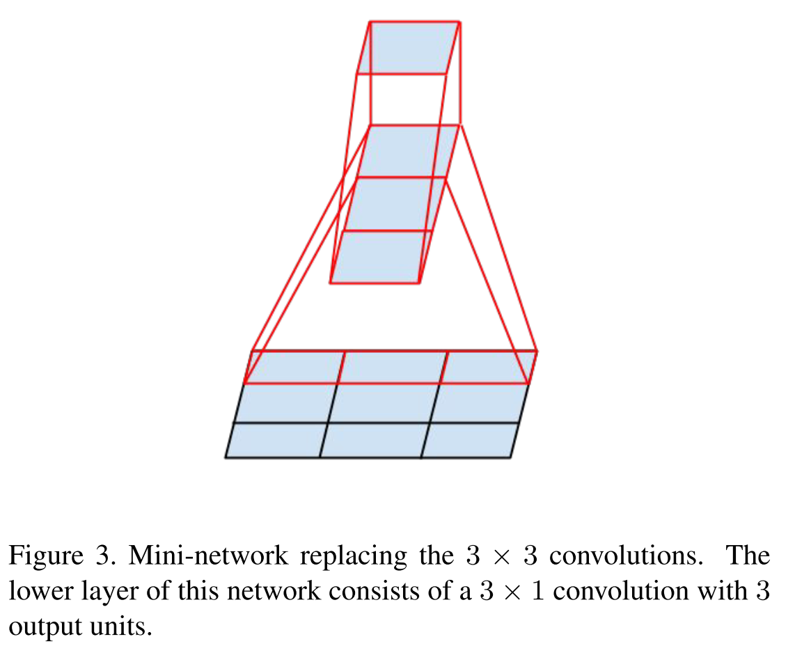
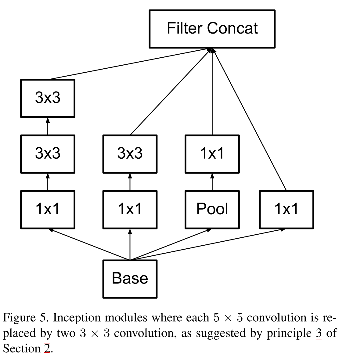
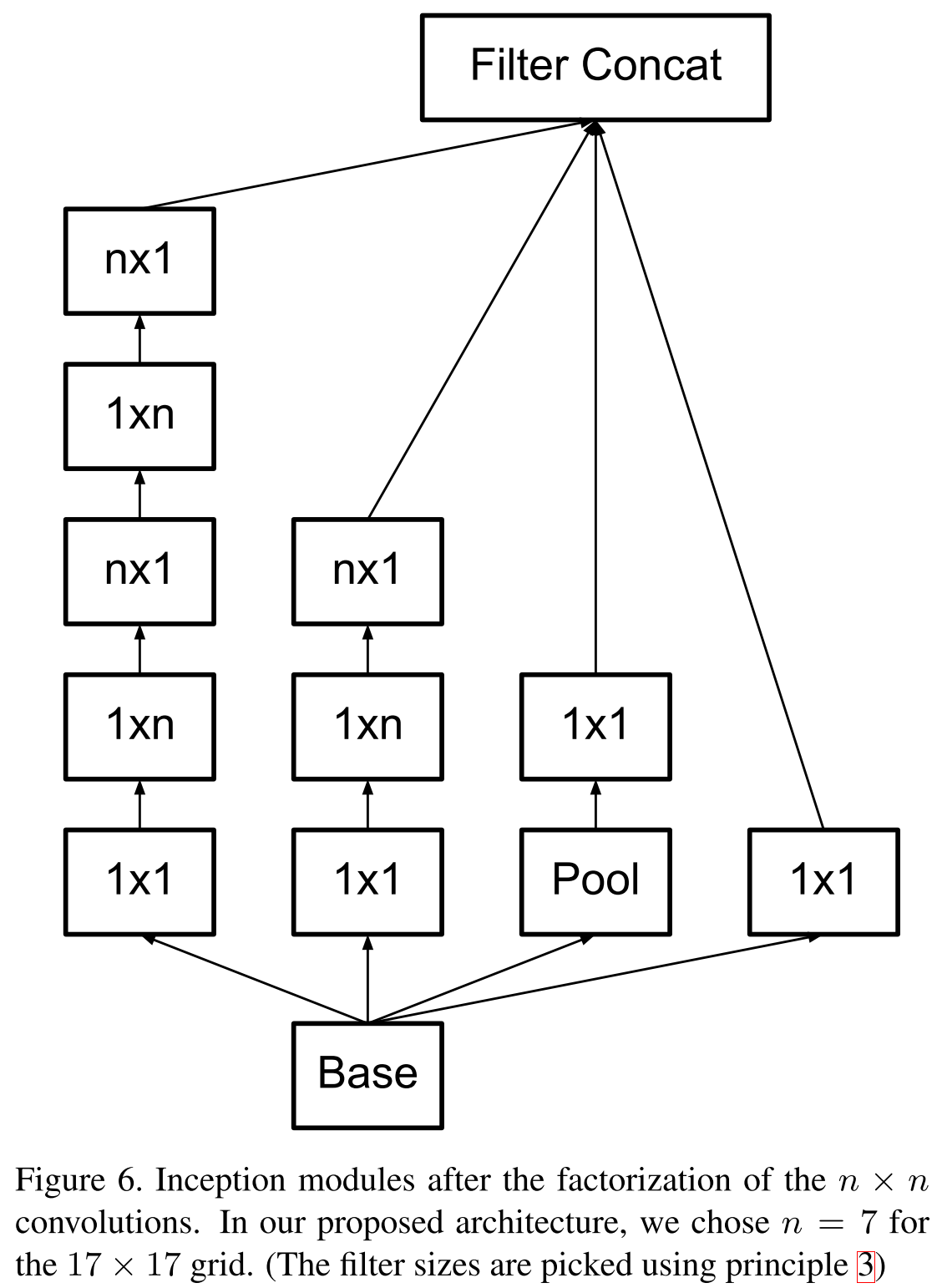
Remember the idea of VGG in 2014, that larger convolutions can be factorized into 3 × 3 bundles? So, Google went even further and factorized all convolutions into N × 1 and 1 × N.
Inception block models
The first is original.
First factorized by the principle of VGG.
New block model.
First factorized by the principle of VGG.
New block model.
As for the bottlenecks, the following scheme is proposed. Suppose if the input dimension
 , and we want to get
  then we first apply convolution of
  filters with step 1 and then affairs pooling. The total complexity of such an operation
  . If you do the pooling first, and then the convolution, then the complexity will fall to
  but then the first principle will be violated. It is proposed to increase the number of parallel branches, to do convolutions with step 2, but at the same time to increase the number of channels twice, then the representative power of the view decreases “smoother”. And for manipulating the depth of the tensor, convolutions of 1 × 1 are used.
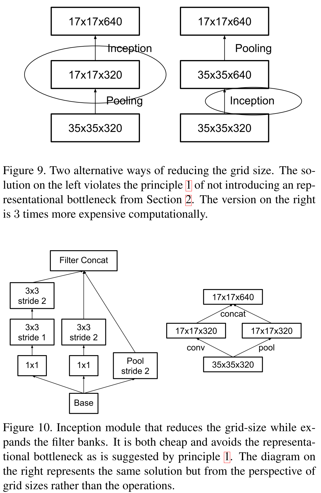
The new model is called Inception V2, and if you add batch normalization , then there will be Inception V3 . By the way, additional classifiers were removed, since it turned out that they do not particularly increase the quality, but can act as a regularizer. But by this time there were already more interesting ways of regularization.
Deep Residual Learning for Image Recognition (10 Dec 2015)
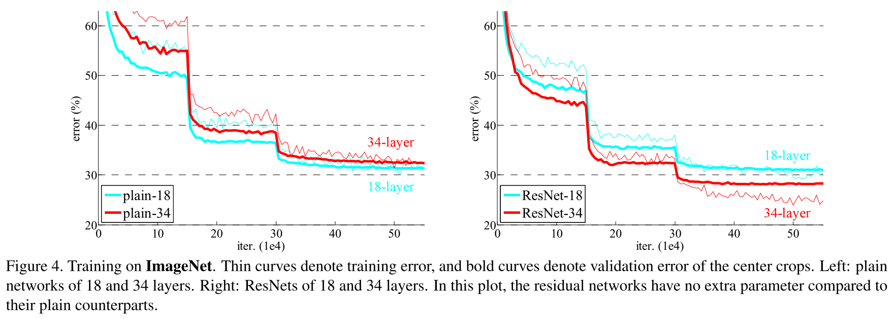
The time has come to study the work of the Chinese division of Microsoft Research, which Google lost in 2015. It has long been noted that if one simply drains more layers, the quality of such a model grows to a certain limit (see VGG-19), and then begins to fall. This problem is called the degradation problem, and the networks obtained by running off more layers are plain, or flat networks. The authors were able to find such a topology in which the quality of the model grows with the addition of new layers.
This is achieved by a simple, at first glance, trick, although it leads to unexpected mathematical results. Thanks to Arnold and Kolmogorov, we and they know that a neural network can approximate almost any function, for example, some complex function
 . Then it is fair that such a network will easily learn the residual-function (in Russian we will call it a residual function):
  . Obviously, our initial objective function will be equal to
  . If we take a certain network, for example, VGG-19, and we attach twenty layers to it, we would like the deep network to behave at least as good as its shallow analogue. The problem of degradation implies that a complex non-linear function
  , obtained by the flow of several layers, must learn the identical transformation, if the previous layers had reached the limit of quality. But this does not happen for some reason, perhaps the optimizer simply does not cope in order to adjust the weights so that the complex nonlinear hierarchical model does the identical transformation. And what if we help her add a shortcut-connection, and it may be easier for the optimizer to make all the weights close to zero, rather than creating an identical transformation. Surely this reminds you of the ideas of boosting.
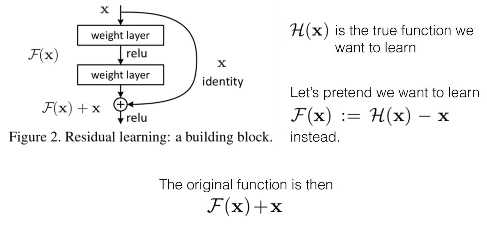
An example of converting a flat network into a residual network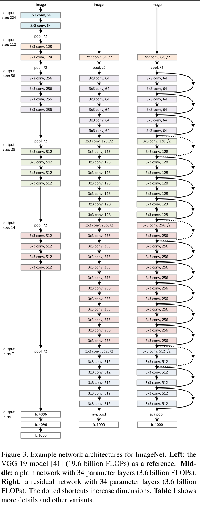
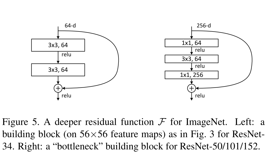
Details of the construction of ResNet-52 at theano / lasagne are described here , but here we only mention that 1 × 1 convolutions are exploited to increase and decrease the dimension, as bequeathed by Google. The network is fully convolution.
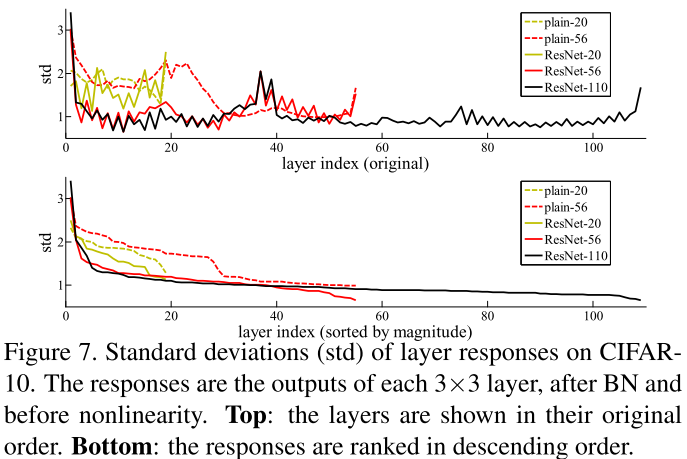
As one of the substantiations of their hypothesis that the residual functions will be close to zero, the authors present a graph of the activation of residual functions depending on the layer and for comparing the activation of layers in flat networks.
And the conclusions from all this are approximately as follows:
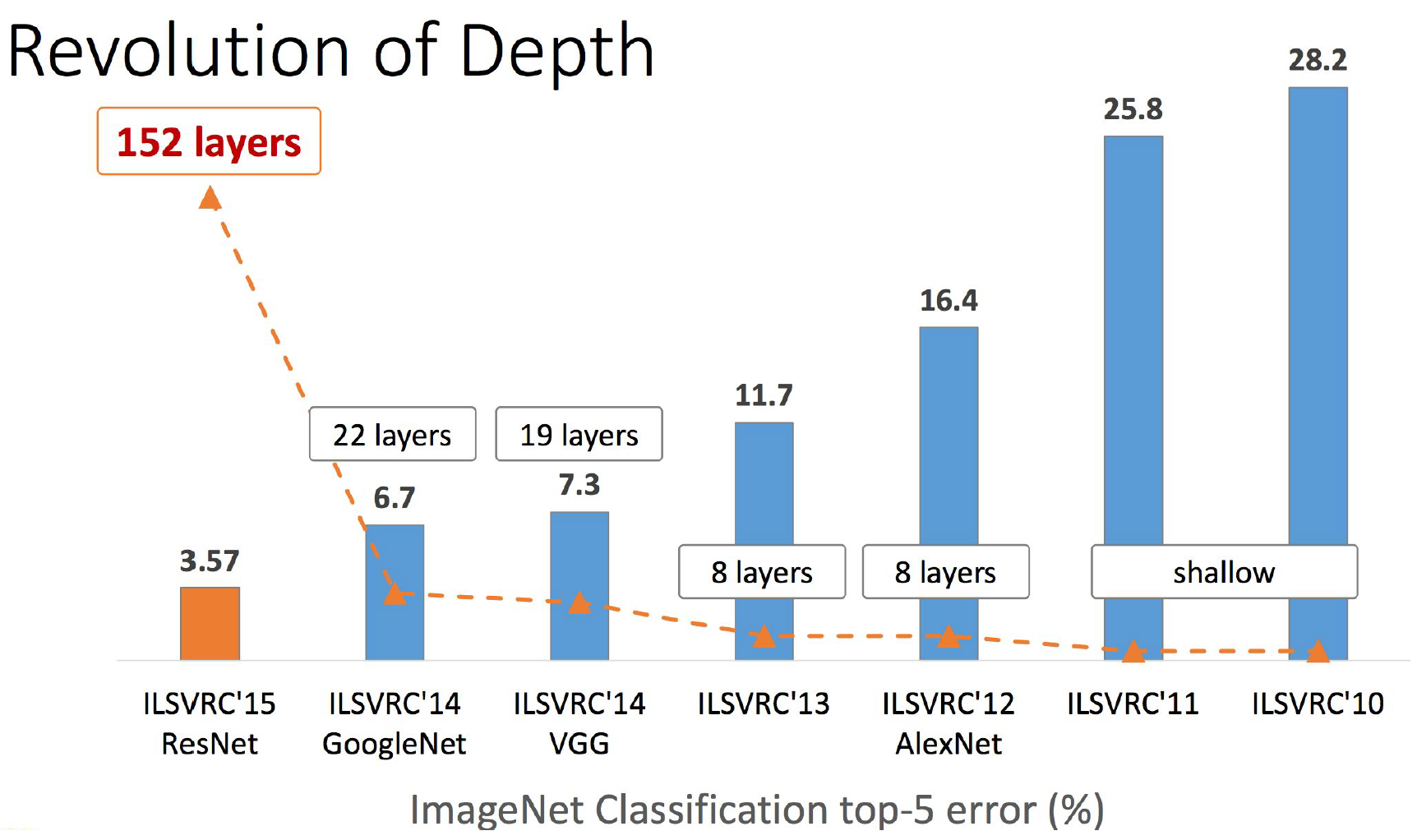
Compare the depth of ResNet and all previous networks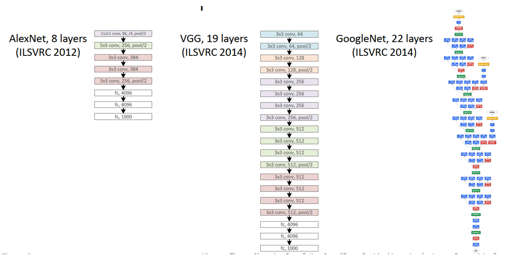
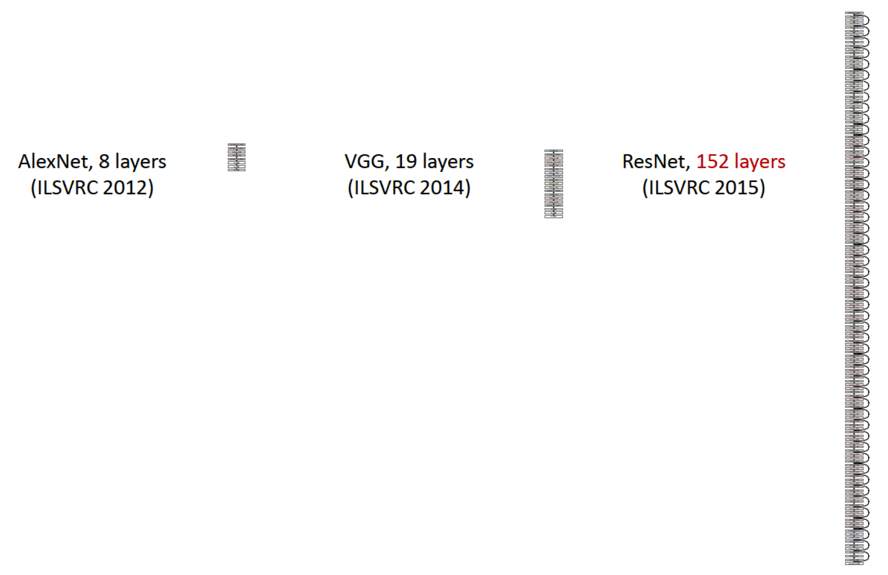
Another interesting slide shows the authors that they have made a breakthrough in the depth / quality of networks. , , , 19- VGG, 152 .
, . , 2016 , . .
ResNet:
Inception-v4, Inception-ResNet and the Impact of Residual Connections on Learning (23 Feb 2016)
, , Inception, ResNet'. , , , . , , . Inception V4 Inception ResNet.
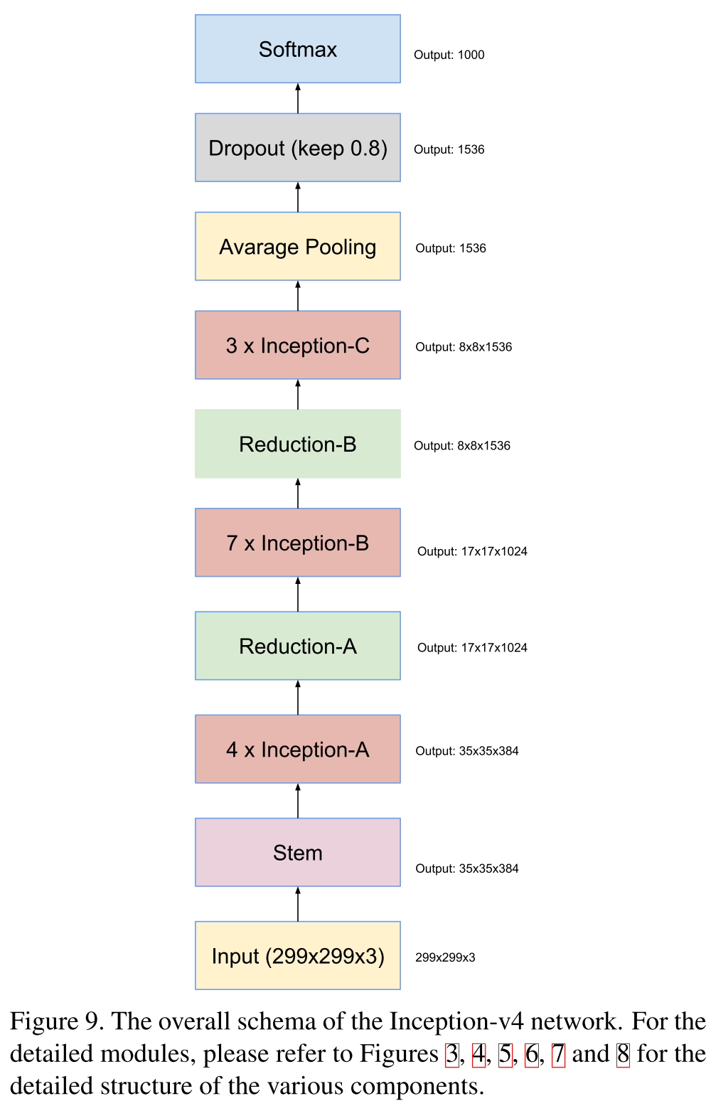
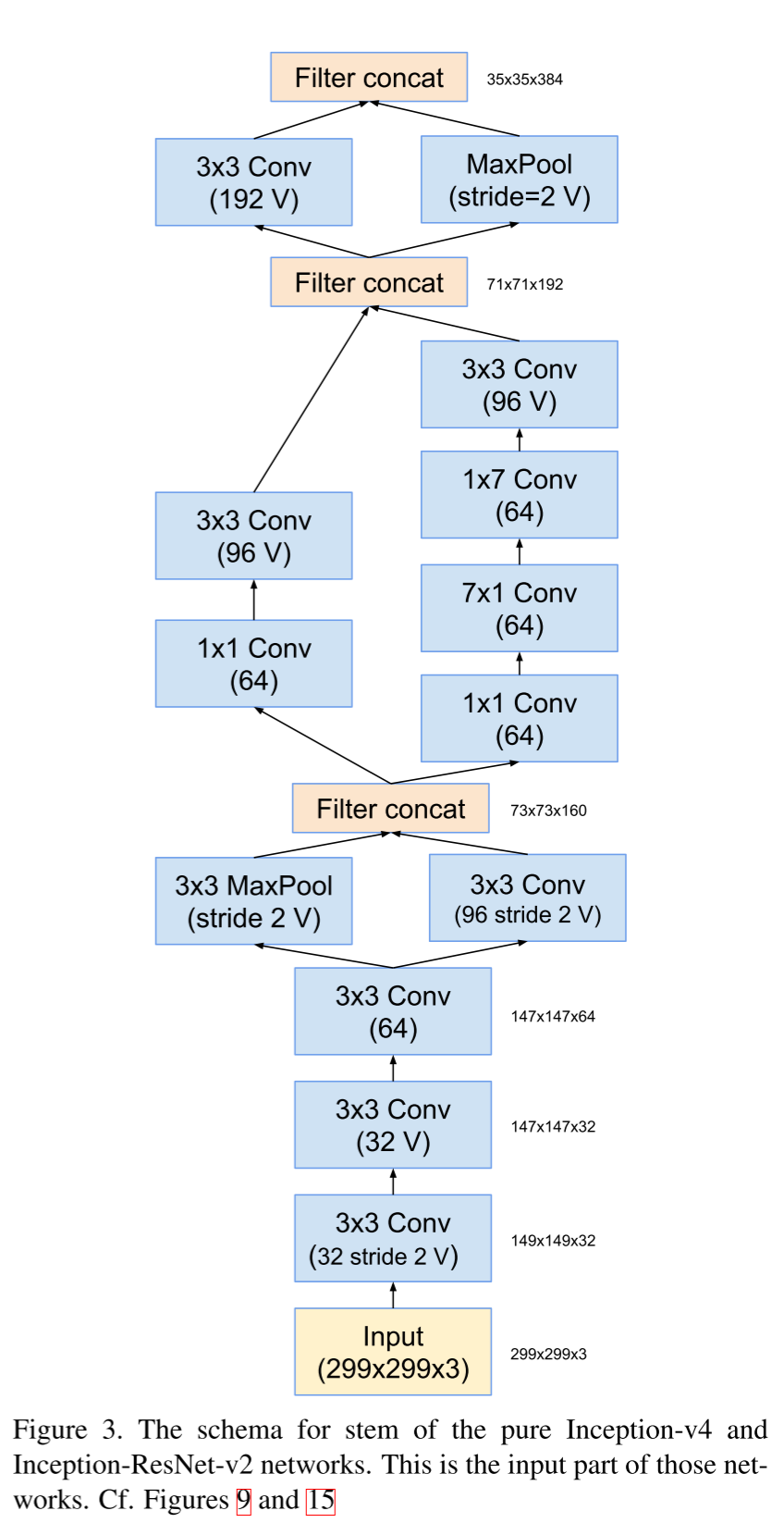
Inception V4 , Inception-. , , 4 , , — , .
Inception V4
The general scheme of the network.
Stem-block.
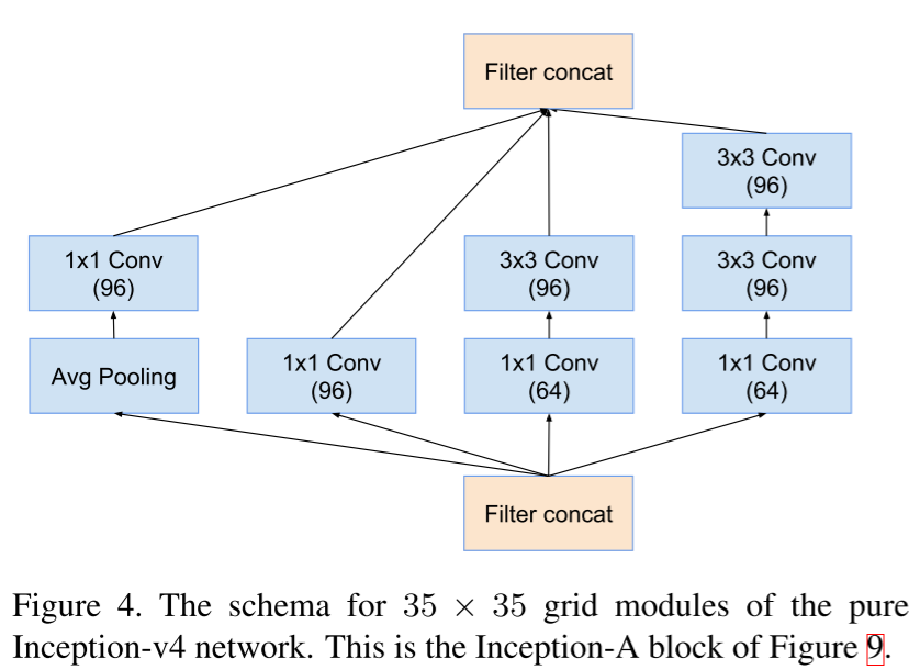
Inception block A.
Stem-block.
Inception block A.
Inception V4 Inception- , shortcut-, Inception ResNet.
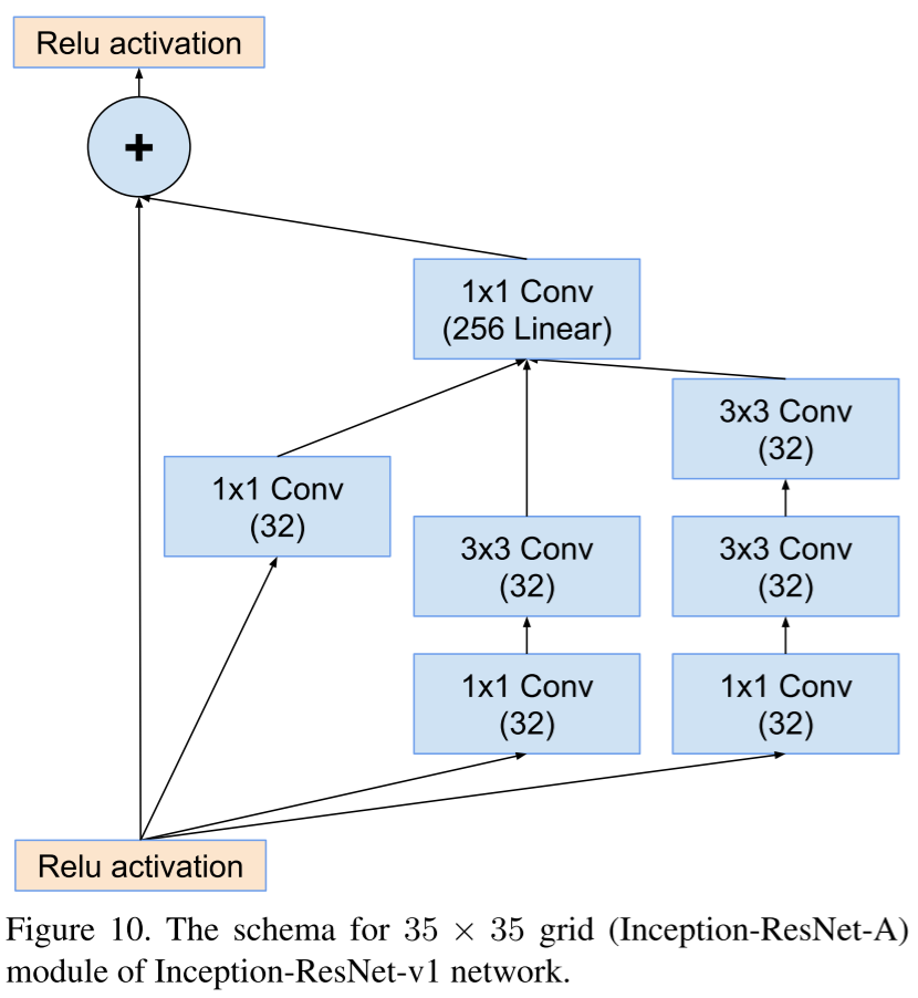
, , , .
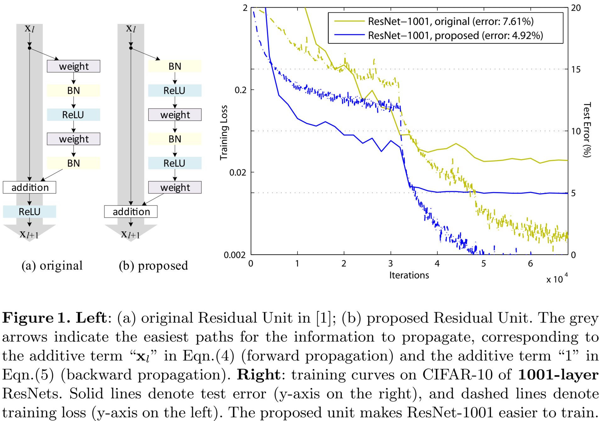
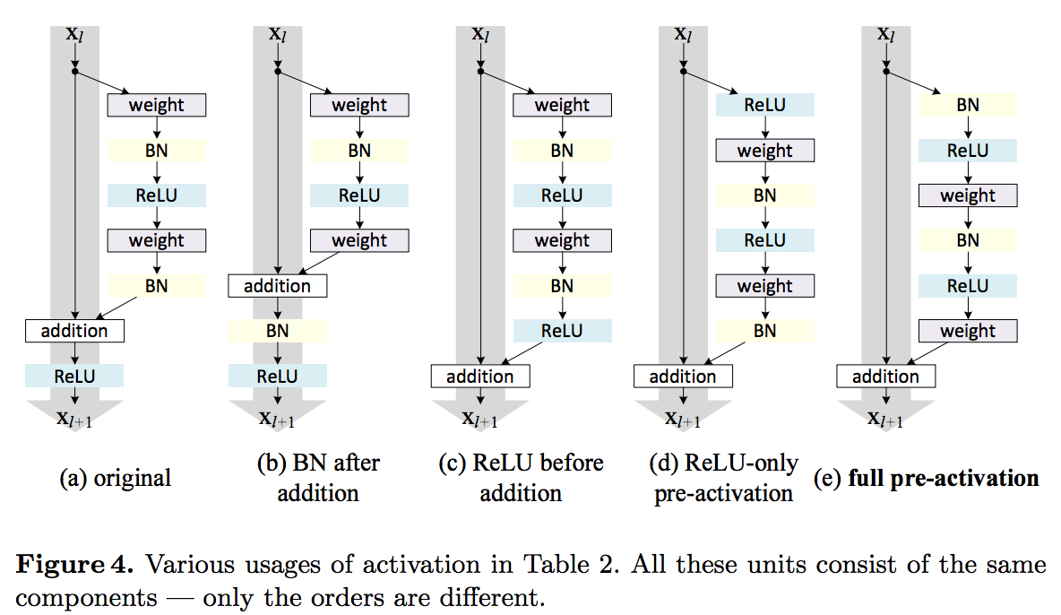
Identity Mappings in Deep Residual Networks (12 Apr 2016)
ResNet, , : . , . . , ; , . , 1001 . , 2014 19- «very deep convolutional neural networks».
. Let be
 — ;
— ; — shortcut connection,
  ;
; — residual network;
 — ;
— ; — .
— .
,
 — , . K , . , . - k , , : . , - . , , vanishing gradients, ,
 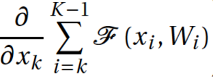 –1. , . , .
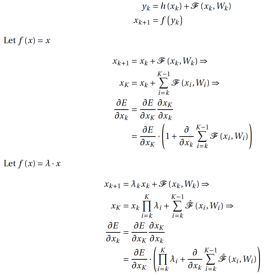
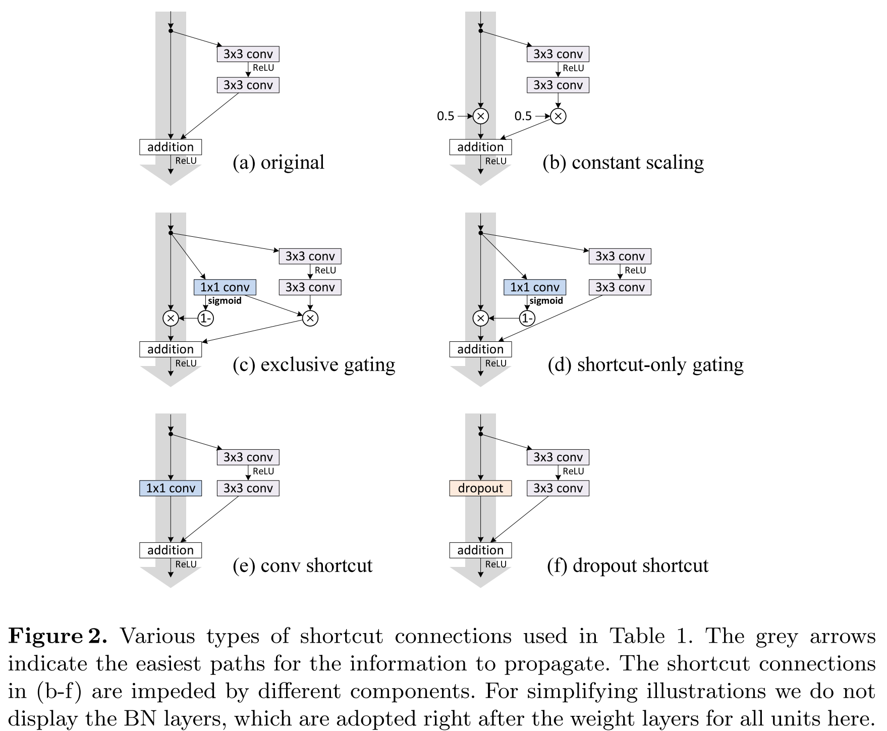
, - ? ,
 . . , . , . .
residual- , , , .
— ( Jürgen Schmidhuber ). LSTM- , 1997 , , ResNet — , LSTM, 1. , — Highway Network . , , , (gate), , .
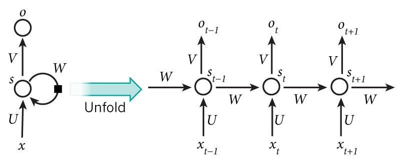
Bridging the Gaps Between Residual Learning, Recurrent Neural Networks and Visual Cortex (13 Apr 2016)
, ResNet RNN. . , , , , , , .
The dark secret of Deep Networks: trying to imitate Recurrent Shallow Networks?
A radical conjecture would be: the effectiveness of most of the deep feedforward neural networks, including but not limited to ResNet, can be attributed to their ability to approximate recurrent computations that are prevalent in most tasks with larger t than shallow feedforward networks. This may offer a new perspective on the theoretical pursuit of the long-standing question “why is deep better than shallow”.
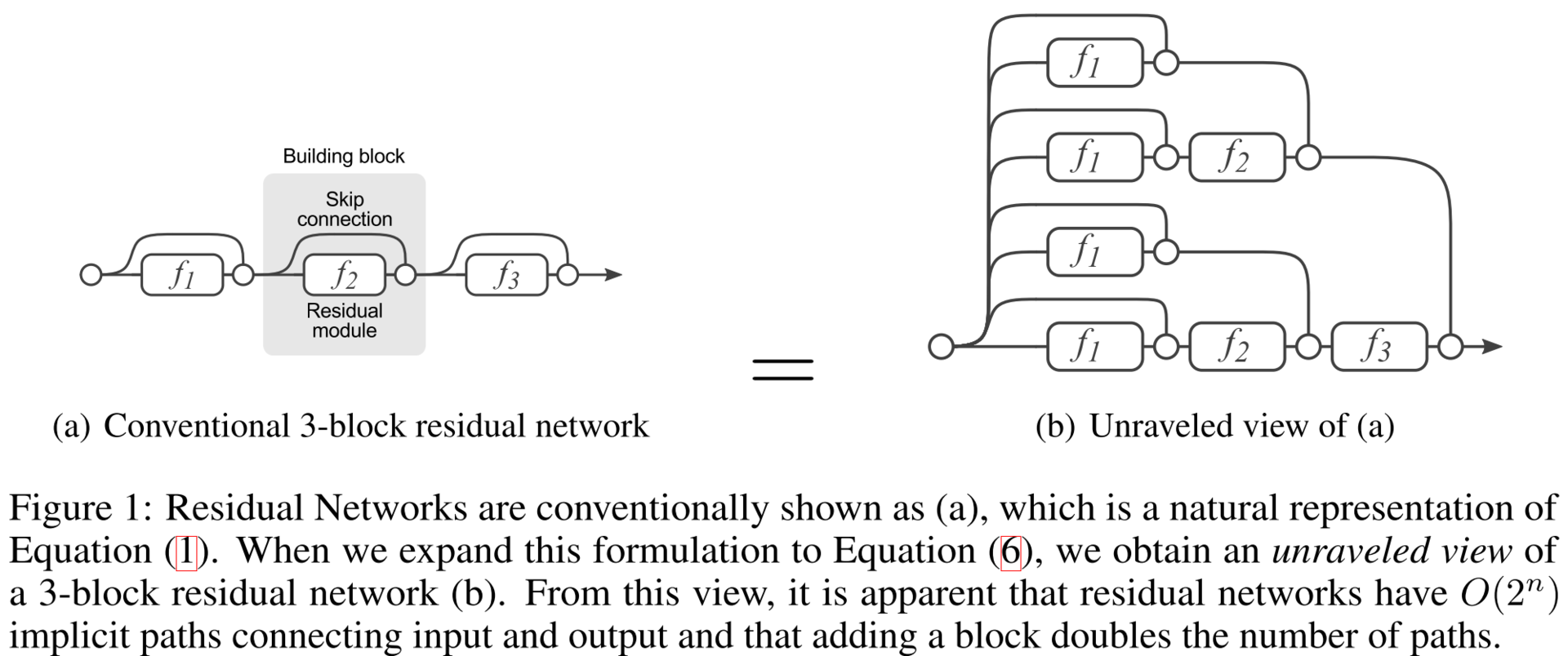
Residual Networks are Exponential Ensembles of Relatively Shallow Networks (20 May 2016)
I'm sure almost all of you are familiar with DropOut, a learning strategy that until recently was the standard for learning deep networks. It was shown that such a strategy is equivalent to learning an exponentially large number of models and averaging the result of forecasting. It turns out the construction of the ensemble learning algorithm. The authors of this article show that ResNet is an ensemble by design. They show it with a series of interesting experiments. First, let's take a look at the expanded version of ResNet, which is obtained if we count two consecutive shortcut connections as one edge of a flowing graph.
You can check this by simply decomposing the formula of the last layer:
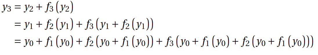
As you can see, the network has grown in another dimension, in addition to the width and depth. The authors say that this is a new third dimension, and they call it multiplicity, in Russian, probably, the closest will be - diversity. It turns out that thanks to Arnold and Kolmogorov, we know that the network needs to grow in width (proven). Thanks to Hinton, we know that adding layers improves the lower variational limit of the likelihood of a model, in general, is also good (proven). And now a new dimension is proposed, that models need to be made diverse, although it is still worth proving.
While there is no evidence, the authors offer the following arguments. After training, in prediction mode, we will remove several layers from the network. It is obvious that all networks before ResNet after such an operation will simply stop working.
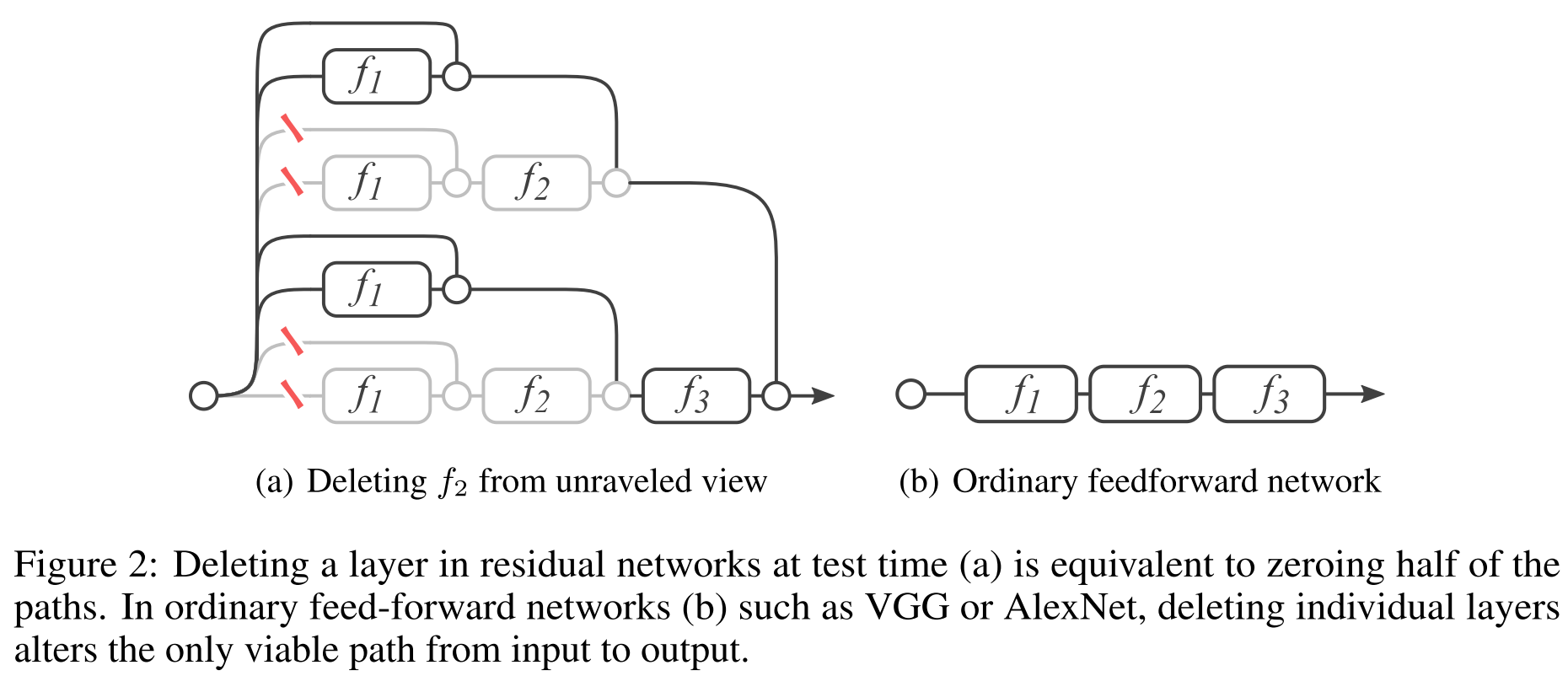
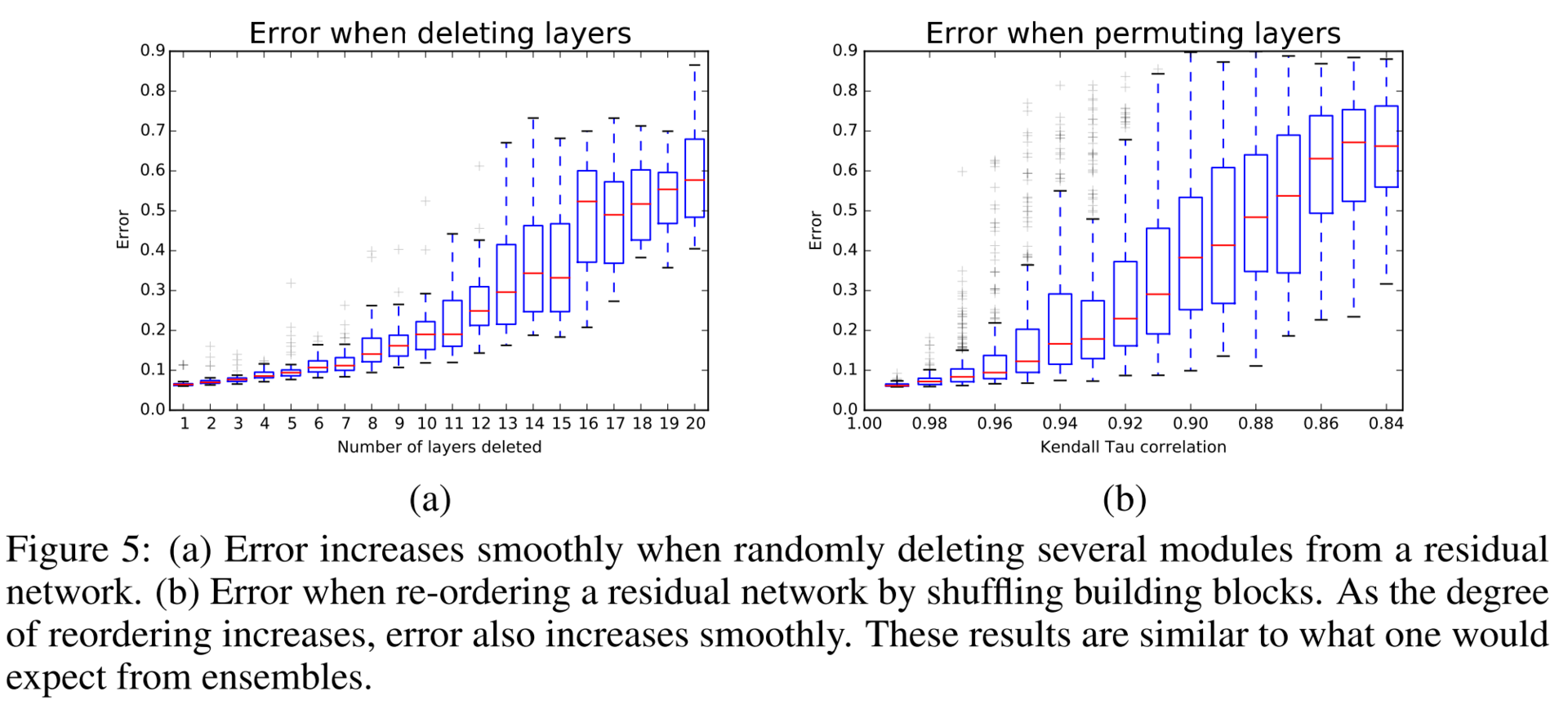
It turns out that the prediction quality of ResNet gradually deteriorates as the number of deleted layers increases. For example, if you remove half of the layers, the quality drops not so dramatically.
It seems that for the sake of trolling, the authors remove several layers from the VGG and from ResNet and compare the quality.
The results are amazing.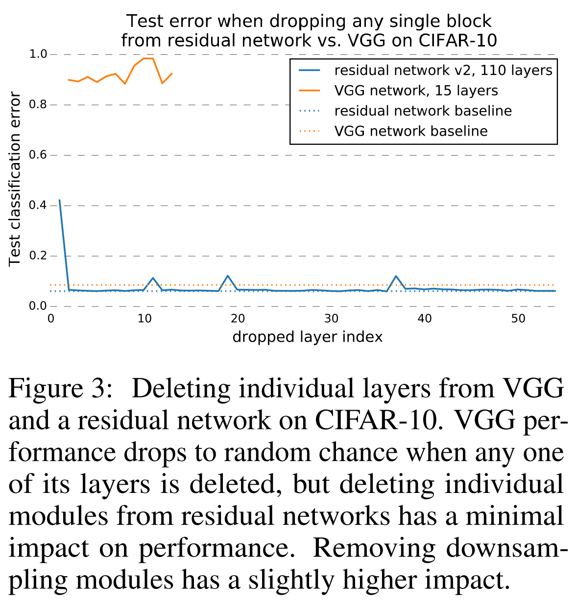
In the next experiment, the authors build the distribution of the absolute values of the gradient obtained from subnets of different lengths. It turns out that for ResNet-50, the effective subnet length is from 5 to 17 layers, they account for almost the entire contribution to the training of the entire model, although they occupy only 45% of all path lengths.
Analysis of the distribution of gradients.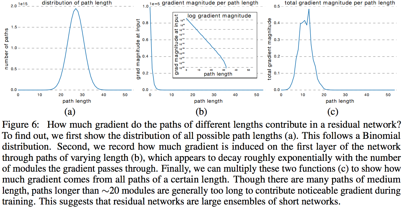
Conclusion
ResNet continues to actively develop, and various groups both try something new and apply proven patterns from the past. For example, create ResNet in ResNet.
- Convolutional Residual Memory Networks (14 Jul 2016)
- Wide Residual Networks (May 23, 2016)
- Depth Dropout: Efficient Training of Convolutional Neural Networks
- Resnet in Resnet: Generalizing Residual Architectures (25 Mar 2016)
- Residual Networks of Residual Networks: Multilevel Residual Networks (9 Aug 2016)
- Multi-Residual Networks (Sep 24, 2016)
- Deep Learning with Separable Convolutions (7 Oct 2016)
- Deep Pyramidal Residual Networks (Oct 10, 2016)
If you read something that is not mentioned in this review, tell us in the comments. To keep track of everything with this stream of new articles is simply not realistic. While this post was moderated on a blog, I managed to add two more new publications to the list. In one, Google talks about the new version of the insector - Xception, and in the second - the pyramidal ResNet.
If you ask someone who is a little versed in neural networks, what types of networks are there, he will say ordinary (fully connected and convolutional) and recurrent. It seems that a theoretical base will soon appear, within which all types of neural networks will belong to the same class. There is a universal approximation theorem, which states that any (almost) function can be approximated by a neural network. A similar theorem for RNN states that any dynamic system can be brought closer by a recurrent network. And now it turns out that RNN can also be approached by a normal network (it remains to prove this, really). In general, we live in an interesting time.
We will see.
Source: https://habr.com/ru/post/311706/
All Articles