How to check causality without experiment?

Today we will talk about establishing causal relationships between phenomena, when it is impossible to conduct an experiment and A / B tests. This is a fairly simple article that will be useful to beginners in statistics and machine learning, or to those who have not thought about such issues before.



Are patients testing a new drug really getting better due to the medication, or would they still recover? Are your sellers really effective, or do they speak with those customers who are already ready to make a purchase? Is Soilent (or an advertising campaign that will cost a company a million dollars) worth your time?

Establishing causal relationships

Causation is incredibly important, but sometimes it is very difficult to establish.

')

A colleague is coming to your table. He kneads himself Soilent - an instant meal replacement, and invites you to try. Soilent looks disgusting, and you wonder what it is useful for. A colleague says that his friends, who consumed this drink for several months, recently ran a marathon. And before that, they did not run? - They ran, last year they also ran a marathon.



In an ideal world, we could conduct an experiment at any time — the gold standard in establishing causal relationships. In reality, this is not always possible. There are doubts about the ethical use of placebo or dangerous untested drugs. Management may not want to try to sell a product to a random set of customers in order to obtain a possible short-term increase in profits, and the team receiving sales bonuses may rebel against this idea.



How to establish causal relationships without applying A / B testing? This is where Propensity Modeling and other causal relationships come into play.

Propensity modeling

So, suppose that we want to simulate the effect of using Soilent using the Propensity Modeling method (the method of selection of control groups according to the correspondence index). To explain his idea, let's conduct a mental experiment.



Imagine that Brad Pitt has a twin brother - an exact copy of it. Brad 1 and Brad 2 wake up at the same time, feed the same way, get the same physical activity. Once Brad 1 manages to buy the last pack of Soilent from a street vendor, and Brad 2 does not have time, so only Brad 1 begins to include Soylent in his diet. In this scenario, any further difference in the health of the twins is most definitely a consequence of the use of Soilent.



Translating the above scenario into real life, one way to assess the effect of Soilent on health would be this:



For each individual using the Soilent, we find no use, comparable in observed characteristics with the first. For example, we could match the Soylent Jay-Z drinker to the non-drinker Kanye West, who uses Natalie Portman — who does not use Keira Knightley, and to the Soilent lover, JK Rowling — doesn’t like Stephanie Meyer.

We measure the Soilent effect as differences between each pair of “twins”.



However, in practice, finding the most similar people is incredibly difficult. Does Jay-Z really fit Kanye, if Jay-Z sleeps on average an hour more than Kanye? Can we match the Jonas Brothers and the One Direction?



Propensity Modeling is a simplification of the above method for selecting control groups. Instead of finding similar individuals on the basis of numerous characteristics, we establish compliance on the basis of a single index characterizing the likelihood that an individual will drink Soilent (“propensity”, “propensity”).



In more detail, the method of selection of control groups based on the compliance index is as follows:

• To begin with, we will determine which of the characteristics of an individual will serve as selection criteria (for example, how a person eats, when he sleeps, where he lives, etc.)
  
  
  
  
• Then we build a probabilistic model (say, logistic regression) based on the selected variables to predict whether the user will drink Soylent. For example, our training sample may consist of many people, some of whom ordered a drink in the first week of March 2016, and we will train the classifier to determine which user will become a user of Soilent.
  
  
  
  
• The probabilistic assessment that an individual becomes a user of our product is called a matching index .
  
  
  
  
• Let's form several groups, for example, let there be only 10 groups: the first includes users with a probability of starting to use Soylent equal to 0-0.1, the second with a probability of 0.1-0.2, etc.
  
  
  
  
• Finally, we compare the adepts and non-adepts of Soilent in each group (for example, we can compare their physical activity, weight, or any other health indicator) in order to evaluate the effect of the drink.

For example, here is a hypothetical distribution of drinkers and non-drinkers of Soilent by age. We can see that those who drink are mostly older, and this interfering factor is one of the reasons why we cannot just carry out a correlation analysis.





After training the model to evaluate the index of compliance and the distribution of users into groups depending on the index, this is how a graph characterizing the influence of a drink on the distance traveled by the consumer can look like a week.





On this hypothetical graph, each of the parts corresponds to a group according to the correspondence index, and the week of the beginning of the impact is the first week of March, when the test groups received the first portions of Soilent. We see that until this week all the subjects ran a good distance. However, after the group receiving the drug starts “treatment,” they start to run more, so that we can evaluate the effect of drinking the drink.

Other causal methods

Without a doubt, there are many other methods for establishing causal relationships between observed phenomena. I will briefly talk about my two loved ones (I originally wrote this post in response to a question with Quora, so I took examples from there).

Building a discontinuous regression model

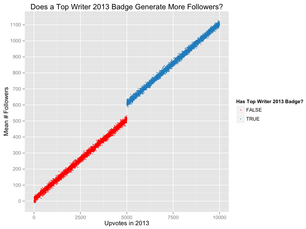
Quora has recently begun to display status icons (badges) on the profile pages of the most active users . Suppose we want to evaluate the effect of this innovation (let's say that since the functionality has already been added, it is impossible to conduct A / B testing). In particular, we are interested in whether the badge of the Top-Author helps the user to acquire more subscribers.



For simplicity, we assume that the badge is issued to each user who received 5,000 or more votes in the previous year. The idea behind the discontinuous regression is that the difference between users who are near the threshold determining whether a badge was received or not received (for example, those who earned 4999 votes and did not receive a badge, and those who earned 5000 votes and received a badge ) can be considered a more or less random event. This means that we can use a sample taken in close proximity to the specified threshold to establish causal relationships.



For example, on an imaginary graph below, a gap in the region of 5,000 subscribers suggests that the Top-Author badge, on average, leads to an increase in the number of subscribers by 100.

Natural experiment

However, finding out the influence of badges on the number of subscribers is not a very interesting question (this is just a simple example). One could ask a deeper question: what happens when a user finds his favorite author? Does the author inspire the reader to create his own materials, further research, thereby encouraging further interaction with the site? How important is contact with the best authors compared to reading a random selection of the best articles?



I studied a similar case when I worked at Google, so instead of an imaginary example with Quora, I’ll tell you better about the work that was done there.



Suppose we want to understand what would happen if we could assign an ideal YouTube channel to each user.

• Does a single-channel enthusiasm lead to an increase in user engagement outside of this channel, for example, because a user visits YouTube to watch their favorite channel, and then it remains to watch something else? This phenomenon is called the multiplicative effect . An example from the world of television: the TV viewer stays at home on Sunday evening specifically to watch the next episode of “Desperate Housewives”, and when the series ends, switch channels in search of something else interesting.
  
  
  
  
• Does a single channel fascination lead to an increase in activity on this channel (the so-called additive effect )?
  
  
  
  
• Does the favorite channel replace other channels in the user’s preferences list? In the end, the time that the user can spend on the site is limited. This is called a neutral effect .
  
  
  
  
• On the contrary, does the time that a user spends on the site decrease with the appearance of the ideal channel, since he spends less time scrolling through and searching for interesting videos? Then we would observe a negative effect.

As always, it would be ideal to conduct A / B testing, but in this case it is impossible: we cannot force the user to fall in love with a certain channel (we can recommend channels to users, but they don’t necessarily like them), we also cannot forbid them watch other channels.



One of the approaches to the study of this effect is a natural experiment — a scenario where the Universe itself generates for us a sample close to a random one. That is his idea.



Consider a user who uploads a new video every Wednesday. One day, he tells subscribers that he will not post new videos for several weeks while he is on vacation.



How will the subscribers respond? Will they stop watching YouTube on Wednesdays, because they usually visit the site just for this channel? Or their activity will not change, since they watch the mentioned channel only when it appears on the main page?



Now, on the contrary, let's imagine that the channel has started downloading new videos on Fridays. Will subscribers start visiting the site also on Fridays? And will they, once logged on to YouTube, watch only a new video, or will it generate a waterfall of search queries and related content?



It turns out that all these scenarios can take place. Here, for example, a calendar of loading of video one popular YouTube channel. As you can see, in 2011 they usually published videos on Tuesdays and Fridays, but at the end of the year they postponed the publication days to Wednesday and Saturday.





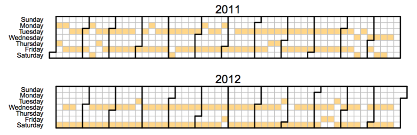
Using this schedule change as a natural experiment that pseudo-randomly cancels viewing of a favorite channel on certain days and introduces it on others, we can try to understand the effect of successfully recommending an ideal channel.



This example of a natural experiment may seem somewhat confusing. The following example may perhaps serve as a more vivid illustration of the idea. Suppose we want to investigate the effect of the magnitude of income on mental health. This article in the New York Times describes a natural experiment in which the Cherokee Indians distributed casino revenues among members of a tribe, thus “accidentally” pulling some of them out of poverty.

Determination of growth factors

Let's go back to Propensity Modeling.



Imagine that we are employees of the development group of our company, and we are faced with the task of finding a way to turn random site visitors into users who return to it every day. What do we do?



If we used Propensity Modeling, the approach would be as follows. We could take a list of events (installation of a mobile application, authorization, subscription to a newsletter or a specific user, etc.) and build a model based on a matching index for each of them. Then we could rank each of the events depending on the effect it has on the user's involvement, and use our ordered list in the next iteration (or use these numbers to convince the management that we need more resources). This is a slightly complicated idea of ​​constructing a regression model of involvement (or a regression model of outflow) of customers and an assessment of the weight of each functionality.



Despite the fact that I am writing this post, I am not a big fan of using Propensity Modeling for many applications in the field of technology (I did not work in the medical field, so I do not have a definite opinion about its usefulness in this area, although I think it is more necessary). I’ll save all my arguments for the next time, I’ll just say that the analysis of causal relationships is an incredibly complex thing, and we can never take into account all the hidden factors that affect the user's attitude. In addition, simply the fact that we have to choose which of the events to include in our model means that we initially believe in the benefit of each of them, while in reality we would like to discover the hidden factors that influence involvement which we would never have thought of.

Conclusion

To summarize: Propensity Modeling is a powerful technique for identifying causal dependencies in the absence of the possibility of conducting a random experiment.



Pure correlation analysis on the basis of observations, after all, can be extremely dangerous. Let me give you my favorite example: if we find that crime is usually higher in cities with the largest police staff, does this mean that we must reduce the number of police officers in order to reduce crime in a country?



As another example, the article on hormone replacement therapy in the framework of the Nurses' Health Study.



And remember that the model is usually as good as the data you give to the input. Taking into account all the hidden variables that may be relevant is a very difficult task, and in a causal model that seems well thought out to you, there may actually be some factors missing (I heard somewhere that Propensity Modeling in the case of nurses led to false conclusions). Therefore, it is always worthwhile to consider alternative approaches to solving your problem, whether there are simpler methods for establishing causal relationships, and maybe it is worth asking users. And even if a random experiment seems like a huge task to you now, an attempt can help to avoid many problems in the future.