ClusterR clustering, part 2
This article focuses on clustering, more precisely, my recently added ClusterR package to CRAN. The details and examples below are mostly based on the Vignette package.
Cluster analysis or clustering is the task of grouping a set of objects so that the objects within one group (called a cluster) are more similar (in one sense or another) to each other than to objects in other groups (clusters). This is one of the main tasks of the research analysis of data and the standard technique of statistical analysis used in various fields, including machine learning, pattern recognition, image analysis, information retrieval, bioinformatics, data compression, computer graphics.
The most well-known examples of clustering algorithms are clustering based on connectivity (hierarchical clustering), clustering based on centers (k-means method, k-medoid method), distribution-based clustering (GMM - Gaussian mixture models) and clustering based on density (DBSCAN - Density-based spatial clustering of applications with noise - spatial clustering of applications with noise based on density, OPTICS - ordering points to identify the clustering structure - ordering points to determine the clustering structure, etc.).
')
In the first part : Gaussian distribution mixture (GMM), k-means method, k-means method in mini-groups.
The k-Medoid Algorithm (L. Kaufman, P. Russo, 1987) is a clustering algorithm that has in common with the k-means algorithm and the Medoid shift algorithm. Alogrhythms of k-medium and k-medoids are separating, and both are trying to minimize the distance between the points, presumably from one cluster and the point designated by the center of this cluster. Unlike the k-means algorithm, the k-medoid method chooses points from a dataset as centers (medoids or standards) and works with an arbitrary metric of distances between points. A useful tool for determining k is the width of the contour. The k-medoid method is more resistant to noise and anomalous values than k-means, because it minimizes the sum of pairwise deviations, rather than the sum of squares of Euclidean distances. A medoid can be defined as a cluster object, whose average deviation from all other objects in the cluster is minimal, i.e. this is the closest point to the cluster center.
The most common implementation of k-medoid clustering is the separation algorithm around the medoids (PAM - Partitioning Around Medoids). RAM has two phases: “build” (BUILD) and “rearrange” (SWAP). In the BUILD phase, the algorithm searches for a good set of source meadoids, and in the SWAP phase, all possible movements between BUILD-medoids and values are made until the objective function stops decreasing (Clustering in an object-oriented environment, A. Struyf, M. Hubert , P. Russo, 1997).
In the ClusterR package, the Cluster_Medoids and Clara_Medoids functions correspond to the PAM (partitioning around medoids) and CLARA (clustering large applications) algorithms.
In the following code example, I use the mushroom data to illustrate how the k-medoid method works with a distance metric other than Euclidean. The mushroom data consists of 23 categorical attributes (including class) and 8124 values. The package documentation has more information about this data.
As input data, the Cluster_Medoids function can also accept a deviation matrix (in addition to the data matrix). In the case of data mushroom, where all variables are categorical (with two or more unique values), it makes sense to use the distance gower . Distance gower applies different functions for different indicators depending on the type (numerical, ordered and unordered list). This deviation metric is implemented in a number of R packages, among others in the cluster package ( daisy function) and the FD package ( gowdis function). I will use the gowdis function from the FD package, since it also allows you to specify user-defined weights as a separate factor.
As previously mentioned, the FD package gowdis function allows the user to set different weights for each individual variable. The weights parameter can be adjusted, for example, using a random search , to achieve better clustering results. For example, using such weights, each individual variable can be improved and adjusted-rand-index (external validation), and average silhouette width (average contour width, internal validation).
CLARA (CLustering LARge Applications - clustering large applications) is the obvious choice for clustering large data sets. Instead of searching for medoids for the entire data set — calculating the incompatibility matrix is also an impossible task — CLARA takes a small sample and applies the PAM algorithm (Partitioning Around Medoids) to generate the best set of medoids for this sample. The quality of the obtained medoids is determined by the average inappropriateness between each object in the dataset and the medoid of its cluster.
The Clara_Medoids function in the ClusterR package uses the same logic, applying the Cluster_Medoids function to each sample. Clara_Medoids takes two more parameters: samples and sample_size . The first determines the number of samples that need to be formed from the original data set, the second - the share of data in each iteration of the sampling (a fractional number between 0.0 and 1.0). It is worth mentioning that the Clara_Medoids function does not accept the incompatibility matrix as an input, unlike the Cluster_Medoids function.
I will apply the Clara_Medoids function to the mushroom dataset previously used, taking the Hamming distance as the dissimilarity metric, and compare the computation time and result with the result of the Cluster_Medoids function. Hamming distance is suitable for mushroom data, because it applies to discrete variables and is defined as the number of attributes that take different values for two compared instances ("Data Mining Algorithms: An Explanation With R", Powell Chikos, 2015, p. 318).
Using the Hamming distance and Clara_Medoids , and Cluster_Medoids return approximately the same result (compared to the results for the gower distance), but the Clara_Medoids function is more than four times faster than the Cluster_Medoids for this data set.
With the results of the last two code fragments, the width of the contour can be plotted using the Silhouette_Dissimilarity_Plot function. It is worth mentioning here that the incompatibility and the width of the contour in the Clara_Medoids function is on the best sample, and not on the entire data set, as for the Cluster_Medoids function.
The implementation of k-medoid functions ( Cluster_Medoids and Clara_Medoids ) took me quite a lot of time, because at first I thought that the initial medoids were initialized in the same way as the centers in the k-means algorithm. Since I did not have access to the book by Kaufman and Rousseau, the cluster package with very detailed documentation helped a lot. It includes both algorithms, and PAM (Partitioning Around Medoids - separation around medoids), and CLARA (CLustering LARge Applications - clustering large applications), if you like, you can compare the results.
In the following code snippet, I’ll compare the cluster’s pam function cluster and Cluster_Medoids of the ClusterR package and the resulting medoids based on the previous quantization example.
For this data set (5625 rows and 3 columns), the Cluster_Medoids function returns the same medoids almost four times faster than the pam function if OpenMP is available (6 streams).
The current version of the ClusterR package is available in my Github repository , and for bug reports, please use this link .
Cluster analysis or clustering is the task of grouping a set of objects so that the objects within one group (called a cluster) are more similar (in one sense or another) to each other than to objects in other groups (clusters). This is one of the main tasks of the research analysis of data and the standard technique of statistical analysis used in various fields, including machine learning, pattern recognition, image analysis, information retrieval, bioinformatics, data compression, computer graphics.
The most well-known examples of clustering algorithms are clustering based on connectivity (hierarchical clustering), clustering based on centers (k-means method, k-medoid method), distribution-based clustering (GMM - Gaussian mixture models) and clustering based on density (DBSCAN - Density-based spatial clustering of applications with noise - spatial clustering of applications with noise based on density, OPTICS - ordering points to identify the clustering structure - ordering points to determine the clustering structure, etc.).
')
In the first part : Gaussian distribution mixture (GMM), k-means method, k-means method in mini-groups.
K-medoid method
The k-Medoid Algorithm (L. Kaufman, P. Russo, 1987) is a clustering algorithm that has in common with the k-means algorithm and the Medoid shift algorithm. Alogrhythms of k-medium and k-medoids are separating, and both are trying to minimize the distance between the points, presumably from one cluster and the point designated by the center of this cluster. Unlike the k-means algorithm, the k-medoid method chooses points from a dataset as centers (medoids or standards) and works with an arbitrary metric of distances between points. A useful tool for determining k is the width of the contour. The k-medoid method is more resistant to noise and anomalous values than k-means, because it minimizes the sum of pairwise deviations, rather than the sum of squares of Euclidean distances. A medoid can be defined as a cluster object, whose average deviation from all other objects in the cluster is minimal, i.e. this is the closest point to the cluster center.
The most common implementation of k-medoid clustering is the separation algorithm around the medoids (PAM - Partitioning Around Medoids). RAM has two phases: “build” (BUILD) and “rearrange” (SWAP). In the BUILD phase, the algorithm searches for a good set of source meadoids, and in the SWAP phase, all possible movements between BUILD-medoids and values are made until the objective function stops decreasing (Clustering in an object-oriented environment, A. Struyf, M. Hubert , P. Russo, 1997).
In the ClusterR package, the Cluster_Medoids and Clara_Medoids functions correspond to the PAM (partitioning around medoids) and CLARA (clustering large applications) algorithms.
In the following code example, I use the mushroom data to illustrate how the k-medoid method works with a distance metric other than Euclidean. The mushroom data consists of 23 categorical attributes (including class) and 8124 values. The package documentation has more information about this data.
Cluster_Medoids
As input data, the Cluster_Medoids function can also accept a deviation matrix (in addition to the data matrix). In the case of data mushroom, where all variables are categorical (with two or more unique values), it makes sense to use the distance gower . Distance gower applies different functions for different indicators depending on the type (numerical, ordered and unordered list). This deviation metric is implemented in a number of R packages, among others in the cluster package ( daisy function) and the FD package ( gowdis function). I will use the gowdis function from the FD package, since it also allows you to specify user-defined weights as a separate factor.
data(mushroom) X = mushroom[, -1] y = as.numeric(mushroom[, 1]) # gwd = FD::gowdis(X) # 'gower' gwd_mat = as.matrix(gwd) # cm = Cluster_Medoids(gwd_mat, clusters = 2, swap_phase = TRUE, verbose = F) | adjusted_rand_index | avg_silhouette_width |
|---|---|
| 0.5733587 | 0.2545221 |
| predictors | weights |
|---|---|
| cap_shape | 4.626 |
| cap_surface | 38.323 |
| cap_color | 55.899 |
| bruises | 34.028 |
| odor | 169.608 |
| gill_attachment | 6.643 |
| gill_spacing | 42.08 |
| gill_size | 57.366 |
| gill_color | 37.938 |
| stalk_shape | 33.081 |
| stalk_root | 65.105 |
| stalk_surface_above_ring | 18.718 |
| stalk_surface_below_ring | 76.165 |
| stalk_color_above_ring | 27.596 |
| stalk_color_below_ring | 26.238 |
| veil_type | 0.0 |
| veil_color | 1.507 |
| ring_number | 37.314 |
| ring_type | 32.685 |
| spore_print_color | 127.87 |
| population | 64.019 |
| habitat | 44.519 |
weights = c(4.626, 38.323, 55.899, 34.028, 169.608, 6.643, 42.08, 57.366, 37.938, 33.081, 65.105, 18.718, 76.165, 27.596, 26.238, 0.0, 1.507, 37.314, 32.685, 127.87, 64.019, 44.519) gwd_w = FD::gowdis(X, w = weights) # 'gower' d_mat_w = as.matrix(gwd_w) # cm_w = Cluster_Medoids(gwd_mat_w, clusters = 2, swap_phase = TRUE, verbose = F) | adjusted_rand_index | avg_silhouette_width |
|---|---|
| 0.6197672 | 0.3000048 |
Clara_medoids
CLARA (CLustering LARge Applications - clustering large applications) is the obvious choice for clustering large data sets. Instead of searching for medoids for the entire data set — calculating the incompatibility matrix is also an impossible task — CLARA takes a small sample and applies the PAM algorithm (Partitioning Around Medoids) to generate the best set of medoids for this sample. The quality of the obtained medoids is determined by the average inappropriateness between each object in the dataset and the medoid of its cluster.
The Clara_Medoids function in the ClusterR package uses the same logic, applying the Cluster_Medoids function to each sample. Clara_Medoids takes two more parameters: samples and sample_size . The first determines the number of samples that need to be formed from the original data set, the second - the share of data in each iteration of the sampling (a fractional number between 0.0 and 1.0). It is worth mentioning that the Clara_Medoids function does not accept the incompatibility matrix as an input, unlike the Cluster_Medoids function.
I will apply the Clara_Medoids function to the mushroom dataset previously used, taking the Hamming distance as the dissimilarity metric, and compare the computation time and result with the result of the Cluster_Medoids function. Hamming distance is suitable for mushroom data, because it applies to discrete variables and is defined as the number of attributes that take different values for two compared instances ("Data Mining Algorithms: An Explanation With R", Powell Chikos, 2015, p. 318).
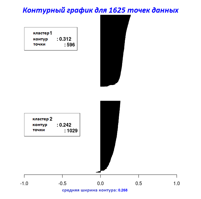
cl_X = X # # Clara_Medoids # for (i in 1:ncol(cl_X)) { cl_X[, i] = as.numeric(cl_X[, i]) } start = Sys.time() cl_f = Clara_Medoids(cl_X, clusters = 2, distance_metric = 'hamming', samples = 5, sample_size = 0.2, swap_phase = TRUE, verbose = F, threads = 1) end = Sys.time() t = end - start cat('time to complete :', t, attributes(t)$units, '\n') # : 3.104652 | adjusted_rand_index | avg_silhouette_width |
|---|---|
| 0.5944456 | 0.2678507 |
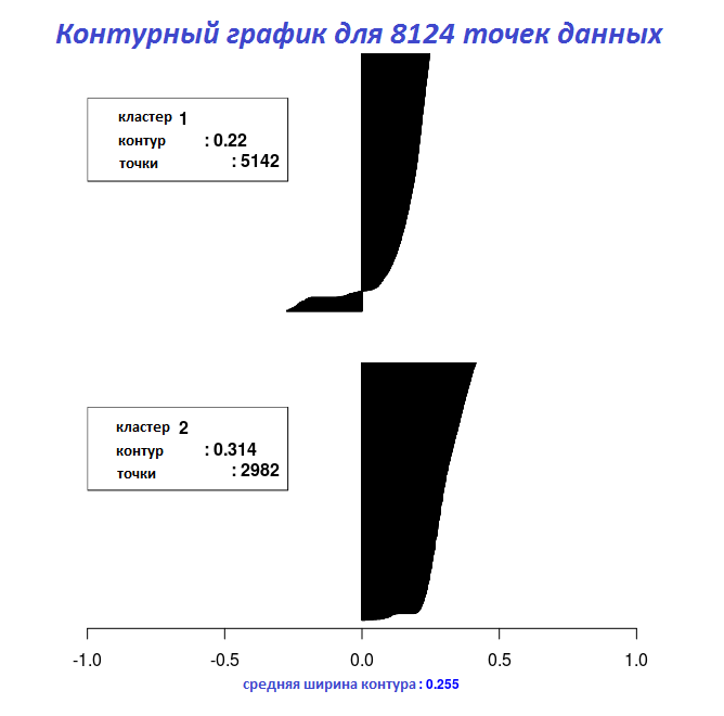
start = Sys.time() cl_e = Cluster_Medoids(cl_X, clusters = 2, distance_metric = 'hamming', swap_phase = TRUE, verbose = F, threads = 1) end = Sys.time() t = end - start cat('time to complete :', t, attributes(t)$units, '\n') # : 14.93423 | adjusted_rand_index | avg_silhouette_width |
|---|---|
| 0.5733587 | 0.2545221 |
Using the Hamming distance and Clara_Medoids , and Cluster_Medoids return approximately the same result (compared to the results for the gower distance), but the Clara_Medoids function is more than four times faster than the Cluster_Medoids for this data set.
With the results of the last two code fragments, the width of the contour can be plotted using the Silhouette_Dissimilarity_Plot function. It is worth mentioning here that the incompatibility and the width of the contour in the Clara_Medoids function is on the best sample, and not on the entire data set, as for the Cluster_Medoids function.
# "Clara_Medoids" Silhouette_Dissimilarity_Plot(cl_f, silhouette = TRUE) # "Cluster_Medoids" Silhouette_Dissimilarity_Plot(cl_e, silhouette = TRUE) Links for k-medoid functions
The implementation of k-medoid functions ( Cluster_Medoids and Clara_Medoids ) took me quite a lot of time, because at first I thought that the initial medoids were initialized in the same way as the centers in the k-means algorithm. Since I did not have access to the book by Kaufman and Rousseau, the cluster package with very detailed documentation helped a lot. It includes both algorithms, and PAM (Partitioning Around Medoids - separation around medoids), and CLARA (CLustering LARge Applications - clustering large applications), if you like, you can compare the results.
In the following code snippet, I’ll compare the cluster’s pam function cluster and Cluster_Medoids of the ClusterR package and the resulting medoids based on the previous quantization example.
#==================================== # pam cluster #==================================== start_pm = Sys.time() set.seed(1) pm_vq = cluster::pam(im2, k = 5, metric = 'euclidean', do.swap = TRUE) end_pm = Sys.time() t_pm = end_pm - start_pm cat('time to complete :', t_pm, attributes(t_pm)$units, '\n') # : 12.05006 pm_vq$medoids # [,1] [,2] [,3] # [1,] 1.0000000 1.0000000 1.0000000 # [2,] 0.6325856 0.6210824 0.5758536 # [3,] 0.4480000 0.4467451 0.4191373 # [4,] 0.2884769 0.2884769 0.2806337 # [5,] 0.1058824 0.1058824 0.1058824 #==================================== # Cluster_Medoids ClusterR 6 ( OpenMP) #==================================== start_vq = Sys.time() set.seed(1) cl_vq = Cluster_Medoids(im2, clusters = 5, distance_metric = 'euclidean', swap_phase = TRUE, verbose = F, threads = 6) end_vq = Sys.time() t_vq = end_vq - start_vq cat('time to complete :', t_vq, attributes(t_vq)$units, '\n') # : 3.333658 cl_vq$medoids # [,1] [,2] [,3] # [1,] 0.2884769 0.2884769 0.2806337 # [2,] 0.6325856 0.6210824 0.5758536 # [3,] 0.4480000 0.4467451 0.4191373 # [4,] 0.1058824 0.1058824 0.1058824 # [5,] 1.0000000 1.0000000 1.0000000 #==================================== # Cluster_Medoids ClusterR #==================================== start_vq_single = Sys.time() set.seed(1) cl_vq_single = Cluster_Medoids(im2, clusters = 5, distance_metric = 'euclidean', swap_phase = TRUE, verbose = F, threads = 1) end_vq_single = Sys.time() t_vq_single = end_vq_single - start_vq_single cat('time to complete :', t_vq_single, attributes(t_vq_single)$units, '\n') # : 8.693385 cl_vq_single$medoids # [,1] [,2] [,3] # [1,] 0.2863456 0.2854044 0.2775613 # [2,] 1.0000000 1.0000000 1.0000000 # [3,] 0.6325856 0.6210824 0.5758536 # [4,] 0.4480000 0.4467451 0.4191373 # [5,] 0.1057339 0.1057339 0.1057339 For this data set (5625 rows and 3 columns), the Cluster_Medoids function returns the same medoids almost four times faster than the pam function if OpenMP is available (6 streams).
The current version of the ClusterR package is available in my Github repository , and for bug reports, please use this link .
Source: https://habr.com/ru/post/311168/
All Articles