“True, true truth and statistics” or “15 probability distributions for all occasions”

Statistics comes to our aid in solving many problems, for example: when there is no possibility to build a deterministic model, when there are too many factors, or when we need to evaluate the likelihood of the constructed model taking into account the available data. Attitude towards statistics is ambiguous. There is an opinion that there are three types of lies: lies, impudent lies and statistics. On the other hand, many “users” of statistics believe it too much, not fully understanding how it works: applying, for example, the Student’s test to any data without checking its normality. Such negligence is capable of causing serious mistakes and turning the “fans” of the Student’s test into haters of statistics. Let us try to put the currents above i and figure out which models of random variables should be used to describe certain phenomena and what kind of genetic relationship exists between them.

First of all, this material will be of interest to students studying probability theory and statistics, although “mature” specialists will be able to use it as a reference book. In one of the following papers, I will show an example of using statistics to build a test assessing the significance of indicators of stock trading strategies.

The paper will consider discrete distributions :

as well as continuous distributions :

At the end of the article will be asked a question for reflection. I will present my thoughts on this in the next article.
')
Some of the cited continuous distributions are special cases of the Pearson distribution .

Discrete distributions

Discrete distributions are used to describe events with non-differentiable characteristics defined at isolated points. Simply put, for events whose outcome can be assigned to a certain discrete category: success or failure, an integer (for example, playing roulette, dice), heads or tails, etc.

Describes the discrete distribution of the probability of occurrence of each of the possible outcomes of the event. As for any distribution (including continuous) for discrete events, the notions of expectation and variance are defined. However, it should be understood that the expectation for a discrete random event is in general unrealizable as the outcome of a single random event, but rather as a quantity to which the arithmetic average of the outcomes of events will tend when their number increases.

In the simulation of discrete random events, combinatorics plays an important role, since the probability of the outcome of an event can be defined as the ratio of the number of combinations giving the desired outcome to the total number of combinations. For example: in the basket are 3 white balls and 7 black ones. When we choose 1 ball from the basket, we can do it in 10 different ways (total number of combinations), but only 3 options for which the white ball will be chosen (3 combinations giving the desired outcome). Thus, the probability of choosing a white ball:

( Bernoulli distribution ).

Samples with and without return should also be distinguished. For example, to describe the probability of choosing two white balls, it is important to determine whether the first ball will be returned to the basket. If not, then we are dealing with a sample without return ( hypergeometric distribution ) and the probability will be as follows:

- the probability to choose a white ball from the initial sample multiplied by the probability to choose the white ball from the remaining ones in the basket again. If the first ball is returned to the basket, then this is a return sample ( Binomial distribution ). In this case, the probability of choosing two white balls will be

.

upstairs

Bernoulli distribution

(taken from here )

If we formalize the basket example as follows: let the outcome of the event can take one of two values 0 or 1 with probabilities

and

accordingly, then the probability distribution of obtaining each of the proposed outcomes will be called the Bernoulli distribution:

$Bin_ {p, q} \ left (x \ right) = \ begin {cases} q, x = 0 \\ p, x = 1 \ end {cases}$

According to the established tradition, the outcome with a value of 1 is called “success”, and the outcome with a value of 0 is called “failure”. Obviously, getting the outcome "success or failure" comes with a probability

.

The expectation and variance of the Bernoulli distribution:

$E \ {Bin_ {p, q} \} = p \ \ \ \ \ left (1.1.2 \ right)$

$D \ {Bin_ {p, q} \} = pq = p \ left (1-p \ right) \ \ \ \ \ left (1.1.3 \ right)$

upstairs

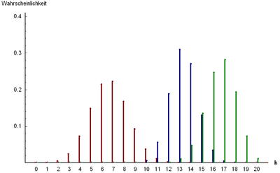
Binomial distribution

(taken from here )

amount

success in

tests, the outcome of which is distributed according to Bernoulli with probability of success

(example with the return of the balls in the basket), described by the binomial distribution:

$B_ {n, p} (k) = C ^ k_np ^ kq ^ {n-k} \ \ (1.2.1)$

Where $C ^ k_n = {n! \ Over {k! (N-k)!}}$ - number of combinations of

.

In other words, the binomial distribution describes the sum of

independent random variables capable of Bernoulli distribution with probability of success

.
Expectation and variance:

$E \ {B_ {n, p} \} = np \ \ (1.2.2)$

$D \ {B_ {n, p} \} = npq \ \ (1.2.3)$

Binomial distribution is valid only for the sample with the return, that is, when the probability of success remains constant for the entire series of tests.

If values

and

have binomial distributions with parameters

and

accordingly, their sum will also be distributed binomially with parameters

.

upstairs

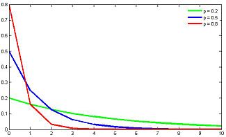
Geometric distribution

(taken from here )

Imagine the situation that we pull the balls out of the basket and return them until the white ball is pulled out. The number of such operations is described by a geometric distribution. In other words: the geometric distribution describes the number of tests

before the first success with the likelihood of success in each trial

. If a

implies a test number in which success occurred, then the geometric distribution will be described by the following formula:

$Geom_p (n) = q ^ {n-1} p \ \ (1.3.1)$

The expectation and variance of the geometric distribution:

$E \ {Geom_p \} = {1 \ over {p}} \ \ \ (1.3.2)$

$D \ {Geom_p \} = {q \ over {p ^ 2}} \ \ \ (1.3.3)$

The geometrical distribution is genetically related to the exponential distribution, which describes a continuous random variable: the time before an event occurs, with a constant intensity of events. Geometric distribution is also a special case of a negative binomial distribution .

upstairs

Pascal distribution (negative binomial distribution)

(taken from here )

The distribution of Pascal is a generalization of the geometric distribution: describes the distribution of the number of failures

in independent trials, the outcome of which is distributed according to Bernoulli with probability of success

before offensive

success in the amount. With

we get the geometric distribution for

$NB_ {r, p} (k) = C ^ k_ {k + r-1} p ^ rq ^ k \ \ (1.4.1)$

Where $C ^ k_n = {n! \ Over {k! (N-k)!}}$ - number of combinations of

.

The expectation and variance of the negative binomial distribution:

$E \ {NB_ {r, p} \} = {rq \ over {p}} \ \ \ (1.4.2)$

$D \ {NB_ {r, p} \} = {rq \ over {p ^ 2}} \ \ \ (1.4.3)$

The sum of independent random variables distributed by Pascal is also distributed by Pascal: let

has a distribution

, but

. Let also

and

independent, then their amount will have distribution

upstairs

Hypergeometric distribution

(taken from here )

So far, we have considered examples of samples with a return, that is, the probability of outcome did not change from trial to trial.

Now consider the situation without returning and describe the probability of the number of successful samples from the aggregate with a previously known number of successes and failures (a known number of white and black balls in the basket, trump cards in the deck, defective parts in the game, etc.).

Let the total population contain

objects of which

marked as “1” and

as "0". We will consider the choice of the object with the label “1” as success, and with the label “0” as failure. We will carry out n tests, and the selected objects will no longer participate in further tests. Probability of occurrence

success will obey the hypergeometric distribution:

$HG_ {N, D, n} (k) = {C ^ k_DC ^ {nk} _ {N-D} \ over {C ^ n_N}} \ \ (1.5.1)$

Where $C ^ k_n = {n! \ Over {k! (N-k)!}}$ - number of combinations of

.

Expectation and variance:

$E \ {HG_ {N, D, n} \} = {nD \ over {N}} \ \ (1.5.2)$

$D \ {HG_ {N, D, n} \} = n {D \ over {N}} {N-D \ over {N}} {N-n \ over {N-1}} \ \ (1.5.3)$

upstairs

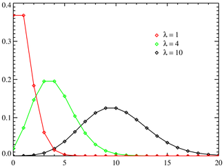
Poisson distribution

(taken from here )

The Poisson distribution differs significantly from the distributions discussed above by its “subject” area: now it is not the likelihood of one or another test outcome that is considered, but the intensity of events, that is, the average number of events per unit of time.

Poisson distribution describes the probability of occurrence

independent events over time

with an average intensity of events

$P _ {\ lambda, t} (k) = {\ left (\ lambda t \ right) ^ k \ over {k!}} E ^ {- \ lambda t} \ \ \ (1.6.1)$

The expectation and variance of the Poisson distribution:

$E \ {P _ {\ lambda, t} \} = \ lambda t \ \ \ (1.6.2)$

$D \ {P _ {\ lambda, t} \} = \ lambda t \ \ \ (1.6.3)$

The variance and the expectation of the Poisson distribution are identically equal.

The Poisson distribution , combined with the exponential distribution describing the time intervals between the onset of independent events, form the mathematical basis of the theory of reliability.

upstairs

Continuous distribution

Continuous distributions, as opposed to discrete ones, are described by probability density functions (distributions)

, defined, in general, at some intervals.

If the probability density is known for

and the transformation is defined

, the probability density for y can be obtained automatically:

$f_y (y) = f \ left (g ^ {- 1} (y) \ right) \ left | {dg ^ {- 1} \ over {dy}} (y) \ right | \ \ \ (2.0.1 )$

subject to uniqueness and differentiability

.

Probability density

sums of random variables

and

(

a) with distributions

and

described by convolution

and

$h (z) = \ int f (t) g (z-t) dt = (f * g) (z) \ \ \ (2.0.2)$

If the distribution of the sum of random variables belongs to the same distribution as the terms, such a distribution is called infinitely divisible. Examples of infinitely divisible distributions: normal , chi-square , gamma , Cauchy distribution .

Probability density

products of random variables x and y (

a) with distributions

and

can be calculated as follows:

$h (z) = \ int f (t) g (z / t) dt \ \ \ (2.0.3)$

Some of the distributions below are special cases of the Pearson distribution, which, in turn, is a solution to the equation:

${df \ over {dx}} (x) = {a_0 + a_1x \ over {b_0 + 2b_1x + b_2x ^ 2}} f (x) \ \ \ (2.0.4)$

Where

and

- distribution parameters. There are 12 types of Pearson distribution, depending on the values of the parameters.

The distributions that will be discussed in this section have close relationships with each other. These relationships are expressed in the fact that some distributions are special cases of other distributions, or they describe transformations of random variables that have other distributions.

The diagram below shows the relationship between some of the continuous distributions that will be considered in this paper. In the diagram, solid arrows show the transformation of random variables (the beginning of the arrow indicates the initial distribution, the end of the arrow indicates the resultant), and the dotted one shows the generalization ratio (the beginning of the arrow indicates the distribution, which is a special case of the one pointed to by the end of the arrow). For particular cases of the Pearson distribution over the dotted arrows, the corresponding type of Pearson distribution is indicated.

The following overview of distributions covers many cases that occur in data analysis and process modeling, although, of course, it does not contain absolutely all of the distributions known to science.

upstairs

Normal distribution (Gaussian distribution)

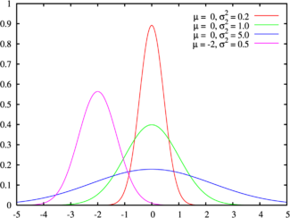
(taken from here )

Probability density of normal distribution

with parameters

and

described by the Gauss function:

$f (x) = {1 \ over {\ sigma \ sqrt {2 \ pi}}} e ^ {(x- \ mu) ^ 2 \ over {2 \ sigma ^ 2}} \ \ \ (2.1.1)$

If a

and

then this distribution is called standard.

The expectation and variance of the normal distribution:

$E \ {N _ {\ mu, \ sigma} \} = \ mu \ \ \ (2.1.2)$

$D \ {N _ {\ mu, \ sigma} \} = \ sigma ^ 2 \ \ \ (2.1.3)$

The domain of definition of a normal distribution is the set of valid numbers.

The normal distribution is the Pearson Type VI distribution.

The sum of squares of independent normal quantities has a chi-squared distribution , and the ratio of independent Gaussian quantities is distributed along Cauchy .

Normal distribution is infinitely divisible: the sum of normally distributed values

and

with parameters

and

accordingly also has a normal distribution with parameters

where

and

.

The normal distribution well models the values describing natural phenomena, the noise of a thermodynamic nature and measurement errors.

In addition, according to the central limit theorem, the sum of a large number of independent terms of the same order converges to the normal distribution, regardless of the distributions of the terms. Due to this property, the normal distribution is popular in statistical analysis, many statistical tests are calculated on normally distributed data.

The z-test is based on the infinite divisibility of the normal distribution. This test is used to test the equality of the expectation of a sample of normally distributed values to a certain value. The value of the variance must be known . If the variance value is unknown and is calculated on the basis of the analyzed sample, then a t-test is used based on the student's distribution .

Suppose we have a sample of n independent normally distributed quantities

out of population with standard deviation

we hypothesize that

. Then the magnitude $z = {\ bar {X} - \ mu \ over {\ sigma \ sqrt {n}}}$ will have a standard normal distribution. By comparing the obtained z value with the quantiles of the standard distribution, one can accept or reject the hypothesis with the required level of significance.

Due to the widespread distribution of the Gauss, many researchers who do not know the statistics very well forget to check the data for normality, or estimate the distribution density graph “by the eye”, blindly thinking that they are dealing with Gaussian data. Accordingly, boldly applying tests designed for normal distribution and getting completely incorrect results. Probably, from here the rumor about statistics as the most terrible kind of lie went.

Consider an example: we need to measure the resistance of a set of resistors of a certain value. Resistance is of a physical nature, it is logical to assume that the distribution of resistance deviations from the nominal will be normal. Measured, we obtain a bell-shaped probability density function for measured values with a mode in the vicinity of the resistors nominal value. Is this a normal distribution? If yes, then we will search for defective resistors using Student's test , or z-test, if we know the distribution variance in advance. I think that many will do just that.

But let's take a closer look at the resistance measurement technology: resistance is defined as the ratio of the applied voltage to the flowing current. We measured current and voltage with instruments, which, in turn, have normally distributed errors. That is, the measured values of current and voltage are normally distributed random variables with expected values corresponding to the true values of the measured values. This means that the obtained resistance values are distributed in Cauchy , and not in Gauss.

The Cauchy distribution only resembles a seemingly normal distribution, but has heavier tails. So the proposed tests are inappropriate. We need to build a test based on the Cauchy distribution or calculate the square of resistance, which in this case will have a Fisher distribution with parameters (1, 1).

to the scheme
upstairs

Chi-square distribution

(taken from here )

Distribution

describes the amount

squares of random variables

each of which is distributed according to standard normal law

$\ chi ^ 2_n (x) = {{\ left (1 \ over 2 \ right)} ^ {k \ over 2} \ over {\ Gamma \ left ({k \ over {2}} \ right)}} x ^ {{k \ over 2} -1} e ^ {- {x \ over 2}} \ \ \ (2.2.1)$

Where

- the number of degrees of freedom $x = \ sum \ limits_ {i = 1} ^ n {X ^ 2_i}$ .

Distribution expectation and variance

$E \ {\ chi ^ 2_n \} = n \ \ \ (2.2.2)$

$D \ {\ chi ^ 2_n \} = 2n \ \ \ (2.2.3)$

The domain is the set of non-negative natural numbers.

is an infinitely divisible distribution. If a

and

- distributed over

and have

and

degrees of freedom respectively, their sum will also be distributed over

and have

degrees of freedom.

is a special case of the gamma distribution (and therefore, the Pearson type III distribution) and a generalization of the exponential distribution . The ratio of values distributed over

distributed by Fisher .

On distribution

based on Pearson's acceptance criterion. Using this criterion, one can verify the reliability of a sample of a random variable to a certain theoretical distribution.

Suppose we have a sample of some random variable

. Based on this sample, we calculate the probabilities

hitting values

intervals (

). Let also there is an assumption about the analytical expression of the distribution, in accordance with which, the probabilities of hitting the selected intervals should be

. Then the magnitudes

will be distributed according to normal law.

Will give

to standard normal distribution:

,
Where $m = {1 \ over n} \ sum \ limits_ {i = 1} ^ n {D_i}$ and $S = \ sqrt {{1 \ over {n-1}} \ sum \ limits_ {i = 1} ^ n {D_i ^ 2}}$ .

Derived values

have a normal distribution with parameters (0, 1), and therefore, the sum of their squares is distributed over

with

degree of freedom. The decrease in the degree of freedom is associated with an additional restriction on the sum of the probabilities of values falling into the intervals: it must be equal to 1.

Comparing the value

with quantiles of distribution,

you can accept or reject the hypothesis about the theoretical distribution of data with the required level of significance.

to the scheme
upstairs

Student's t-distribution (t-distribution)

( )

t-: , ( f- ). , - .

T- z- , .

:

n , ,

. - .

, :

$T_{n}(x)={\Gamma \left({n+1 \over 2}\right) \over {\sqrt{n \pi}\Gamma \left({n \over 2}\right)\left(1+{x^2 \over n}\right)^{n+1 \over 2}}}\ \ \ (2.3.1)$

Where

— - .

.

:

$E\{T_{n}\}=0\ \ \ (2.3.2)$

$D\{T_{n}\}={n \over {n-2}}\ \ \ (2.3.3)$

.

upstairs

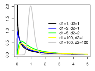
(taken from here )

Let be

and

independent random variables with a chi-square distribution with degrees of freedom

and

respectively.Then the magnitude

will have a Fisher distribution with degrees of freedom

, and the magnitude will have a Fisher

distribution with degrees of freedom

.
Fisher distribution is defined for valid non-negative arguments and has a probability density:

$F_{n_1,n_2}(x)={\sqrt{ (n_1x)^{n_1}n_2^{n_2}\over {(n_1x+n_2)^{n_1+n_2}}} \over {xB\left({n_1 \over 2},{n_2 \over 2} \right)}}\ \ \ (2.4.1)$

The expectation and variance of the Fisher distribution:

$E\{F_{n_1,n_2}\}={n_2 \over {n_2-2}}\ \ \ (2.4.2)$

$D\{F_{n_1,n_2}\}={2n_2^2(n_1+n_2-2) \over {n_1(n_2-2)^2(n_2-4)}}\ \ \ (2.4.3)$

The expectation is defined for

, and the variance is for

.

, , (f-, ).

F-:

and

respectively. .

, .

upstairs

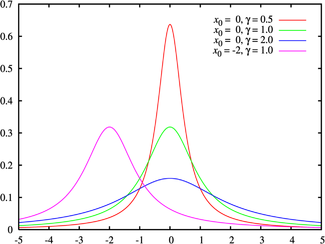
(taken from here )
The Cauchy distribution describes the ratio of two normally distributed random variables. Unlike other distributions, the expectation and variance are not defined for the Cauchy distribution. The shift

and scale factors are used to describe the distribution.

$C_{x_0,\gamma}(x)={1\over{\pi \gamma \left(1+\left({x-x_0\over {\gamma}} \right)^2 \right)}}\ \ \ (2.5.1)$

The Cauchy distribution is infinitely divisible: the sum of independent random variables distributed over Cauchy is also distributed along Cauchy.

to the scheme
upstairs

Exponential (exponential) distribution and Laplace distribution (double exponential, double exponential)

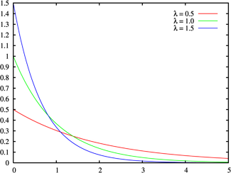
(taken from here ) The

exponential distribution describes the time intervals between independent events occurring with an average intensity

. . .

, , , , — , .

- ( n=2), , - . - - 2- , .

, .

— .

:

$E_\lambda(x)=\lambda e^{-\lambda x}\ \ \ (2.6.1)$

.

:

$E\{E_\lambda\}={1 \over \lambda} \ \ \ (2.6.2)$

$E\{E_\lambda\}={1 \over \lambda^2} \ \ \ (2.6.3)$

, ,

, , .

( )

, , «» . , , .

$L_{\alpha,\beta}(x)={\alpha \over 2}e^{-\alpha \left|x-\beta\right|} \ \ \ (2.6.4)$

Where

— ,

— .

:

$E\{L_{\alpha, \beta}\}=\beta\ \ \ (2.6.5)$

$D\{L_{\alpha, \beta}\}={2 \over {\alpha^2}}\ \ \ (2.6.6)$

, , , , , , ..

upstairs

(taken from here )

Weibull distribution is described by a probability density function of the following form:

$W_{k, \lambda}(x)={k \over {\lambda}}\left({x \over {\lambda}}\right)^{k-1}e^{-\left({x \over {\lambda}}\right)^k}\ \ \ (2.7.1)$

Where

(

> 0) is the intensity of events (similar to the exponential distribution parameter ), and

is the nonstationarity index (

). With

The Weibull distribution degenerates into an exponential distribution , and in other cases describes the flow of independent events with non-stationary intensity. With

— . : .

, — . , , , ..

:

$E\{W_{k, \lambda}\}=\lambda \Gamma\left(1 + {1 \over k} \right)\ \ \ (2.7.2)$

$D\{W_{k, \lambda}\}=\lambda^2 \left(\Gamma\left(1 + {2 \over k} \right ) - \Gamma\left(1 + {1 \over k} \right )^2\right)\ \ \ (2.7.3)$

Where

— - .

upstairs

- ( )

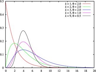
(taken from here )

The gamma distribution is a generalization of the chi-squared distribution and, accordingly, the exponential distribution . The sums of squares of normally distributed quantities , as well as the sums of quantities distributed over chi-square and exponentially distributed, will have a gamma distribution.

The gamma distribution is a Pearson Type III distribution . The domain of the gamma distribution is natural non-negative numbers.

Gamma distribution is determined by two non-negative parameters.

- the number of degrees of freedom (for the whole value of degrees of freedom, the gamma distribution is called the Erlang distribution) and the scale factor

.

Gamma distribution is infinitely divisible: if magnitudes

and

have distributions

and

accordingly, then

will have distribution

$G_ {k, \ theta} (x) = x ^ {k-1} {e ^ {- {x \ over \ theta}} \ over \ Gamma (k) \ theta ^ k} \ \ \ (2.8.1 )$

Where

- Euler gamma function.

Expectation and variance:

$E \ {G_ {k, \ theta} \} = k \ theta \ \ \ (2.8.2)$

$D \ {G_ {k, \ theta} \} = k \ theta ^ 2 \ \ \ (2.8.3)$

Gamma distribution is widely used to model complex flows of events, the sums of time intervals between events, in economics, queuing theory, in logistics, describes the life expectancy in medicine. It is a kind of analogue of the discrete negative binomial distribution .

to the scheme
upstairs

Beta distribution

(taken from here )

The beta distribution describes the fraction of the sum of two terms that falls on each of them, if the terms are random variables that have a gamma distribution . That is, if the quantities

and

have a gamma distribution

and

will have a beta distribution.

Obviously, the domain of the beta distribution

. The beta distribution is the Pearson Type I distribution.

$B _ {\ alpha, \ beta} = {x ^ {\ alpha -1} (1-x) ^ {\ beta - 1} \ over {B (\ alpha, \ beta)}} \ \ \ (2.9.1 )$

where are the parameters

and

- positive natural numbers,

- Euler beta function.

Expectation and variance:

$E \ {B _ {\ alpha, \ beta} \} = {\ alpha \ over {\ alpha + \ beta}} \ \ \ (2.9.2)$

$D \ {B _ {\ alpha, \ beta} \} = {\ alpha \ beta \ over {(\ alpha + \ beta) ^ 2 (\ alpha + \ beta + 1)}} \ \ \ (2.9.3)$

to the scheme
upstairs

Instead of conclusion

We reviewed 15 probability distributions, which, in my opinion, cover most of the most popular statistical applications.

Finally, a small homework: to assess the reliability of exchange trading systems, use such an indicator as the profit factor. Profit factor is calculated as the ratio of total income to total loss. Obviously, for a revenue-generating system, the profit factor is greater than one, and the higher its value, the more reliable the system.

Question: what is the distribution of the profit factor?

I will present my thoughts on this in the next article.

PS If you want to refer to the numbered formulas from this article, you can use the following link: link_on_statyu #x_y_z, where (xyz) is the number of the formula to which you refer.

Source: https://habr.com/ru/post/311092/

All Articles

“True, true truth and statistics” or “15 probability distributions for all occasions”

Discrete distributions

Bernoulli distribution

Binomial distribution

Geometric distribution

Pascal distribution (negative binomial distribution)

Hypergeometric distribution

Poisson distribution

Continuous distribution

Normal distribution (Gaussian distribution)

Chi-square distribution

Student's t-distribution (t-distribution)

Exponential (exponential) distribution and Laplace distribution (double exponential, double exponential)

- ( )

Beta distribution

Instead of conclusion

More articles: